

Space Physics made EASY










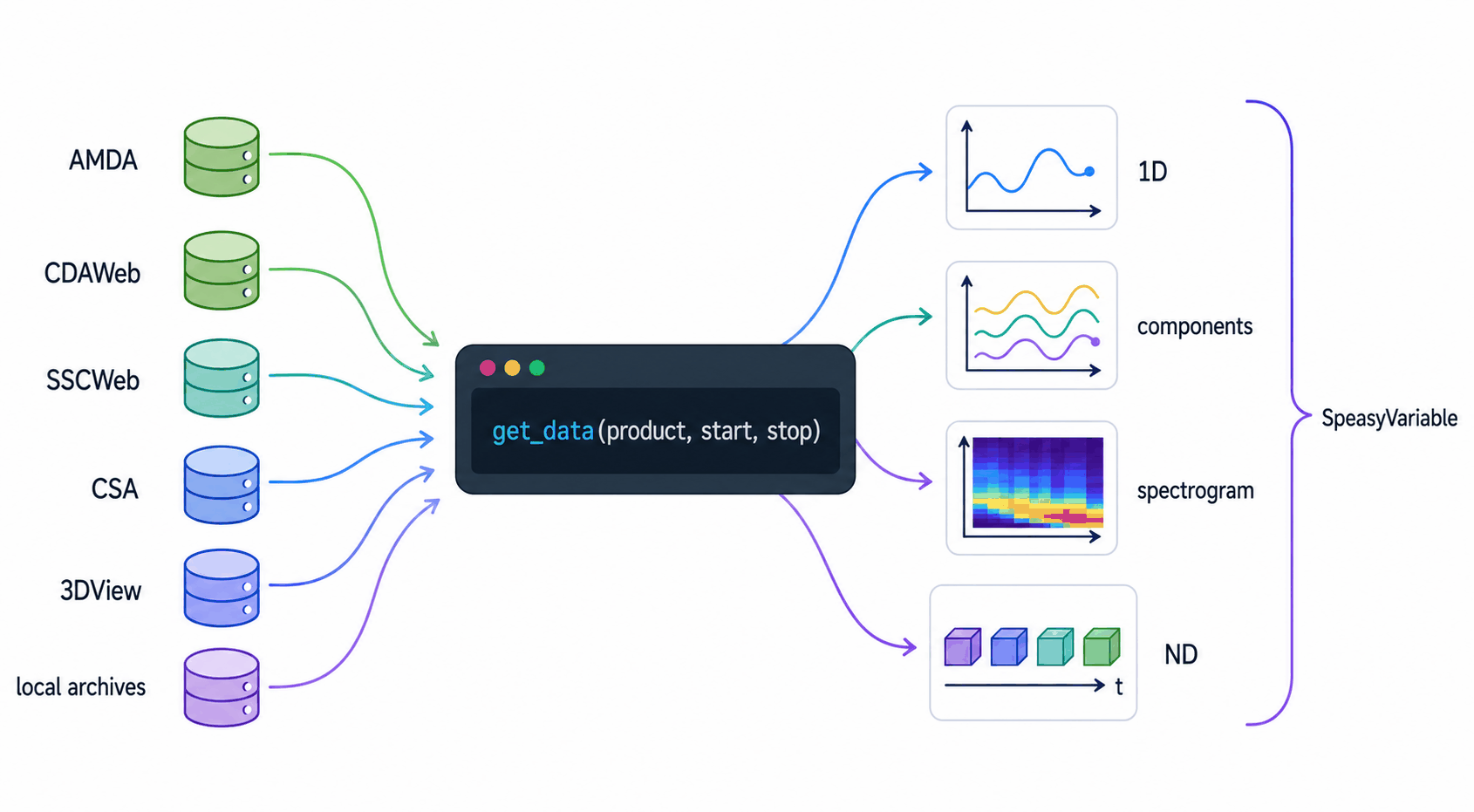
Speasy is a free and open-source Python package that makes it easy to find and load space physics data from a variety of data sources, whether it is online and public such as CDAWEB and AMDA, or any described archive, local or remote. Finding and loading data is where any science project starts. It would seem easy a priori but, considering the diverse array of missions and instruments available nowadays, it proves to be one of the major bottlenecks, especially for students and newcomers. Speasy solves this problem by providing a single, easy-to-use interface to over 70 space missions and 65,000 products.
Don't want to write code? See our graphical interface SciQLop.
Main features
- Simple and intuitive API (
spz.get_data(...)to get them all) - Speasy variables are like Pandas DataFrames with seamless conversion to/from them (as long as the shape is compatible)
- Speasy variables support numpy operations, see numpy operations example below
- Speasy variables filtering and resampling capabilities, see resampling example below
- Also supports Catalogs, TimeTables, Events, and multi-variable Datasets
- Local cache to avoid redundant downloads, backed by pysciqlop-cache (see notes for users upgrading from an older Speasy)
- Uses the SciQLOP ultra fast community cache server (see configuration to tune or disable it)
- Full support of AMDA API
- Can retrieve time-series from AMDA (analysis server at IRAP/CDPP), CDAWeb (NASA/GSFC archive), CSA (ESA Cluster archive) and SSCWeb (NASA orbit/trajectory service); see the data providers documentation for more.
- Support data access from any local or remote archives described by YAML file.
- Also available as Speasy.jl for Julia users
Help us improve Speasy!
We want Speasy to be the best possible tool for space physics research. You can help us by:
- Answering our user survey here.
- Reporting bugs or requesting features here.
- Creating or participating in discussions here.
Your feedback is essential to making Speasy a better tool for everyone.
Quickstart
Installation
Speasy requires Python 3.10 or newer. We recommend installing it with pip inside a virtual environment (more details here, conda works too):
$ python3 -m venv .venv
$ source .venv/bin/activate
$ python -m pip install speasy
# or, without a virtual environment:
$ python -m pip install --user speasy
Troubleshooting: your first get_data calls need internet access (data is then cached locally);
if you are behind a proxy or firewall, see the configuration page.
Examples
Simple request
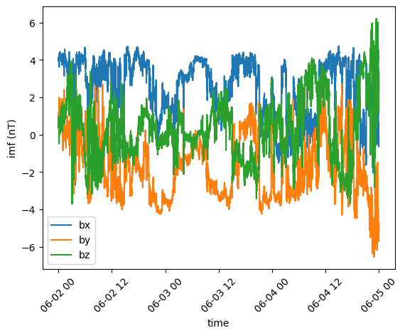
This simple code example shows how easy it is to get data using Speasy. The code imports the Speasy package and defines a variable named ace_mag. This variable stores the data for the ACE IMF (interplanetary magnetic field) product, for the time period from June 2, 2016 to June 5, 2016. The code then uses the Speasy plot() function to plot the data.
import speasy as spz
ace_mag = spz.get_data('amda/imf', "2016-6-2", "2016-6-5")
ace_mag.plot();
Using the dynamic inventory
Where amda is the data provider and imf is the product ID.
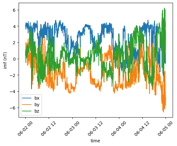
Using the dynamic inventory produces the same result as the previous example, but lets you discover available data through tab-completion in IPython, Jupyter notebooks, or any Python environment that supports it.
You can discover product ids by browsing spz.inventories.tree.<provider> (e.g. spz.inventories.tree.amda)
with tab-completion, or programmatically via spz.inventories.flat_inventories.<provider>.
See the concepts page for more details.
import speasy as spz
amda_tree = spz.inventories.data_tree.amda
ace_mag = spz.get_data(amda_tree.Parameters.ACE.MFI.ace_imf_all.imf, "2016-6-2", "2016-6-5")
ace_mag.plot();
Plotting multiple time series on a single figure
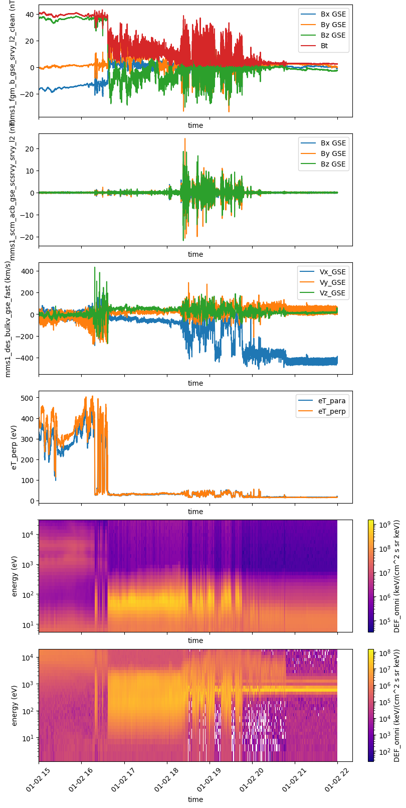
This code example shows how to use Speasy to plot multiple time series of space physics data from the MMS1 spacecraft on a single figure, with a shared x-axis. The code imports the Speasy package and the Matplotlib plotting library. It then creates a figure with six subplots, arranged in a single column. Next, it defines a list of products and axes to plot. Finally, it iterates over the list of products and axes, plotting each product on the corresponding axis. The code uses the Speasy get_data() function to load the data for each product, and the replace_fillval_by_nan() function to replace any fill values (placeholders for missing data) with NaNs. The products plotted here include magnetic field measurements from the FGM (fluxgate magnetometer) instrument, expressed in GSE (a geocentric coordinate frame).
Note: Speasy may transparently fall back between access methods (direct archive, web service, community cache); messages such as "switching to web service" are informational, not errors.
import speasy as spz
import matplotlib.pyplot as plt

fig = plt.figure(figsize=(8, 16), layout="constrained")
gs = fig.add_gridspec(6, hspace=0, wspace=0)
axes = gs.subplots(sharex=True)

plots = [
    (spz.inventories.tree.cda.MMS.MMS1.FGM.MMS1_FGM_SRVY_L2.mms1_fgm_b_gse_srvy_l2_clean, axes[0]),
    (spz.inventories.tree.cda.MMS.MMS1.SCM.MMS1_SCM_SRVY_L2_SCSRVY.mms1_scm_acb_gse_scsrvy_srvy_l2 , axes[1]),
    (spz.inventories.tree.cda.MMS.MMS1.DES.MMS1_FPI_FAST_L2_DES_MOMS.mms1_des_bulkv_gse_fast, axes[2]),
    (spz.inventories.tree.cda.MMS.MMS1.DES.MMS1_FPI_FAST_L2_DES_MOMS.mms1_des_temppara_fast, axes[3]),
    (spz.inventories.tree.cda.MMS.MMS1.DES.MMS1_FPI_FAST_L2_DES_MOMS.mms1_des_tempperp_fast, axes[3]),
    (spz.inventories.tree.cda.MMS.MMS1.DES.MMS1_FPI_FAST_L2_DES_MOMS.mms1_des_energyspectr_omni_fast, axes[4]),
    (spz.inventories.tree.cda.MMS.MMS1.DIS.MMS1_FPI_FAST_L2_DIS_MOMS.mms1_dis_energyspectr_omni_fast, axes[5])
]

def plot_product(product, ax):
    values = spz.get_data(product, "2019-01-02T15", "2019-01-02T22")
    values.replace_fillval_by_nan().plot(ax=ax)

for p in plots:
    plot_product(p[0], p[1])
Requesting multiple products and intervals at once
More complex requests like this one are supported:
The result is a list per product, each holding one variable per requested interval.
import speasy as spz
products = [
    spz.inventories.tree.amda.Parameters.Wind.SWE.wnd_swe_kp.wnd_swe_vth,
    spz.inventories.tree.amda.Parameters.Wind.SWE.wnd_swe_kp.wnd_swe_pdyn,
    spz.inventories.tree.amda.Parameters.Wind.SWE.wnd_swe_kp.wnd_swe_n,
    spz.inventories.tree.cda.Wind.WIND.MFI.WI_H2_MFI.BGSE,
    spz.inventories.tree.ssc.Trajectories.wind,
]
intervals = [["2010-01-02", "2010-01-02T10"], ["2009-08-02", "2009-08-02T10"]]
data = spz.get_data(products, intervals)
Numpy operations
Speasy variables support numpy operations, as shown in this example. The code imports the Speasy package and the NumPy library, and uses the Speasy get_data() function to load the magnetic field data for the MMS1 spacecraft for the time period from January 1, 2017 to January 1, 2017. The code then uses the NumPy sqrt() and sum() functions to compute the norm of the magnetic field vector. Finally, the code uses the NumPy allclose() function to check if the computed norm is close to the provided total magnetic field norm (Bt) values.
import speasy as spz
import numpy as np
mms1_products = spz.inventories.tree.cda.MMS.MMS1
b = spz.get_data(mms1_products.FGM.MMS1_FGM_SRVY_L2.mms1_fgm_b_gsm_srvy_l2, '2017-01-01T02:00:00', '2017-01-01T02:00:15')
b.replace_fillval_by_nan(inplace=True)  # replace fill values by NaN
bt = b["Bt"]
b = b["Bx GSM", "By GSM", "Bz GSM"]
computed_norm = np.sqrt(np.sum(b ** 2, axis=1))
print(f"Type of b: {type(b)}")
print(f"Type of computed_norm: {type(computed_norm)}")
print(f"Type of bt: {type(bt)}")
print("Is the computed norm close to the provided total magnetic field norm?", bool(np.allclose(computed_norm, bt)))
Type of b: <class 'speasy.products.variable.SpeasyVariable'> Type of computed_norm: <class 'speasy.products.variable.SpeasyVariable'> Type of bt: <class 'speasy.products.variable.SpeasyVariable'> Is the computed norm close to the provided total magnetic field norm? True
Resampling
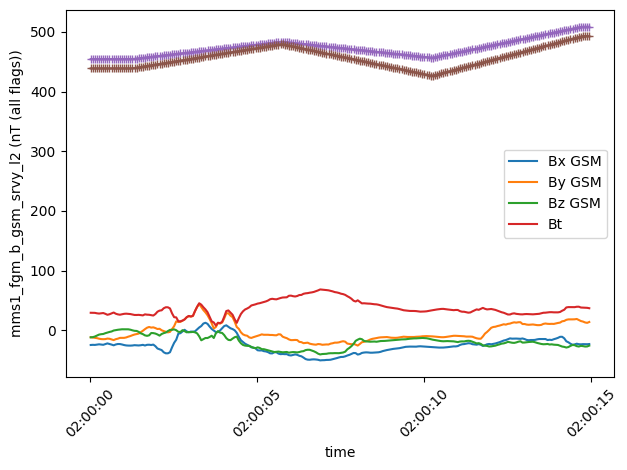
Speasy provides a simple way to filter and resample data. In this example, the code imports the Speasy package and the Matplotlib plotting library. It then uses the Speasy get_data() function to load the magnetic field and temperature data for the MMS1 spacecraft for the time period from January 1, 2017 to January 1, 2017. The code then uses the Speasy interpolate() function to interpolate the temperature data to match the magnetic field data sampling rate. Finally, the code plots the magnetic field and temperature data on the same figure.
import speasy as spz
from speasy.signal.resampling import interpolate
import matplotlib.pyplot as plt
mms1_products = spz.inventories.tree.cda.MMS.MMS1

b, Tperp, Tpara = spz.get_data(
        [
            mms1_products.FGM.MMS1_FGM_SRVY_L2.mms1_fgm_b_gsm_srvy_l2,
            mms1_products.DIS.MMS1_FPI_FAST_L2_DIS_MOMS.mms1_dis_tempperp_fast,
            mms1_products.DIS.MMS1_FPI_FAST_L2_DIS_MOMS.mms1_dis_temppara_fast
        ],
        '2017-01-01T02:00:00',
        '2017-01-01T02:00:15'
    )

Tperp_interp, Tpara_interp = interpolate(b, [Tperp, Tpara])

plt.figure()
ax = b.plot()
plt.plot(Tperp_interp.time, Tperp_interp.values, marker='+')
plt.plot(Tpara_interp.time, Tpara_interp.values, marker='+')
plt.tight_layout()
Documentation and examples
Check out Speasy documentation and examples.
Caveats
- Speasy is not a plotting package. basic plotting capabilities are here for illustration purposes and making quick-and-dirty plots. It is not meant to produce publication ready figures, prefer using Matplotlib directly for example.
Credits
The development of Speasy is supported by the CDPP.
This package was created with Cookiecutter and the audreyr/cookiecutter-pypackage project template.
3 maintainers


Release files for speasy 1.8.2
For a detailed explanation of source distributions (sdists) and built distributions (wheels), please see the package formats documentation.
Source distribution (sdist)
| File | Size | Uploaded | |
|---|---|---|---|
| speasy-1.8.2.tar.gz | 13.3 MB | Details |
Built distribution (wheel)
| File | Interpreter | ABI | Platform | Reset |
|---|---|---|---|---|
| speasy-1.8.2-py3-none-any.whl | Python 3 | none | any | Details |
Total release size: 13.5 MB
Release files / speasy-1.8.2.tar.gz
| Download URL | speasy-1.8.2.tar.gz |
|---|---|
| Size | 13.3 MB |
| Tags | Source |
|
SHA-256 checksum How to use checksums |
aca0b5b8b8258ce1d7a380324c53664567249f968eccc443c7a7a7d23603bd08
|
|
BLAKE2b-256 checksum How to use checksums |
04991765b3623b79bc3d0b32f5024b5a4d6a0bd3fd8e94834a8e7b355788e265
|
| Upload date | |
|
Uploaded using Trusted Publishing? What is trusted publishing? |
No |
| Uploaded via |
twine/7.0.0 CPython/3.10.21
|
Release files / speasy-1.8.2-py3-none-any.whl
| Download URL | speasy-1.8.2-py3-none-any.whl |
|---|---|
| Size | 159.4 kB |
| Tags | Python 3 |
|
SHA-256 checksum How to use checksums |
a57a6cc261b37dc43dcc69fadbd74d95a31921d13a4a3c635fb09812af4461b8
|
|
BLAKE2b-256 checksum How to use checksums |
c8378b9c0e37e3b799007060859745b56e453d9a41964342bf8b1346baac90fb
|
| Upload date | |
|
Uploaded using Trusted Publishing? What is trusted publishing? |
No |
| Uploaded via |
twine/7.0.0 CPython/3.10.21
|














