
SpeciesNet
An ensemble of AI models for classifying wildlife in camera trap images.
Table of Contents
- Overview
- Running SpeciesNet
- Downloading SpeciesNet model weights directly
- Contacting us
- Citing SpeciesNet
- Output format
- Visualizing SpeciesNet output
- Ensemble decision-making
- Fine-tuning SpeciesNet
- Advanced topics
- Animal picture
Overview
Effective wildlife monitoring relies heavily on motion-triggered wildlife cameras, or “camera traps”, which generate vast quantities of image data. Manual processing of these images is a significant bottleneck. AI can accelerate that processing, helping conservation practitioners spend more time on conservation, and less time reviewing images.
This repository hosts code for running a cascade of two AI models: (1) an object detector that finds objects of interest in wildlife camera images, and (2) an image classifier that classifies those objects to the species level. This approach is used for species recognition in the Wildlife Insights platform.
The object detector used in this ensemble is MegaDetector, which finds animals, humans, and vehicles in camera trap images, but does not classify animals to species level.
The species classifier (SpeciesNet) was trained at Google using a large dataset of camera trap images and an EfficientNet V2 M architecture. It is designed to classify images into one of more than 2000 labels, covering diverse animal species, higher-level taxa (like "mammalia" or "felidae"), and non-animal classes ("blank", "vehicle"). SpeciesNet has been trained on a geographically diverse dataset of over 65M images, including curated images from the Wildlife Insights user community, as well as images from publicly-available repositories.
The full details of the species classifier are discussed in this paper:
Gadot T, Istrate Ș, Kim H, Morris D, Beery S, Birch T, Ahumada J. To crop or not to crop: Comparing whole-image and cropped classification on a large dataset of camera trap images. IET Computer Vision. 2024 Dec;18(8):1193-208.
Running SpeciesNet
Do I have to do all this command line stuff?
No, you don't have to run anything at the command line to use SpeciesNet: there are a number of tools that help you run SpeciesNet on your computer or on cloud-based systems. Details are beyond the scope of this README, but cloud-based systems that support SpeciesNet include Wildlife Insights and Animl. AddaxAI is a popular graphical tool for running SpeciesNet on your computer.
This README, though, is about running SpeciesNet at the command line, so, on to instructions...
Setting up your Python environment
The instructions on this page will assume that you have a Python virtual environment set up. If you have not installed Python, or you are not familiar with Python virtual environments, start with our installing Python page. If you see a prompt that looks something like the following, you're all set to proceed to the next step:

Installing the SpeciesNet Python package
You can install the SpeciesNet Python package via:
pip install speciesnet
If you are on a Mac, and you receive an error during this step, add the "--use-pep517" option, like this:
pip install speciesnet --use-pep517
To confirm that the package has been installed, you can run:
python -m speciesnet.scripts.run_model --help
You should see help text related to the main script you'll use to run SpeciesNet.
Running SpeciesNet
The easiest way to run SpeciesNet is via the "run_model" script, like this:
python -m speciesnet.scripts.run_model --folders "c:\your\image\folder" --predictions_json "c:\your\output\file.json"
Change c:\your\image\folder to the root folder where your images live, and change c:\your\output\file.json to the location where you want to put the output file containing the SpeciesNet results.
This will automatically download and run the detector and the classifier. This command periodically logs output to the output file, and if this command doesn't finish (e.g. you have to cancel or reboot), you can just run the same command, and it will pick up where it left off.
These commands produce an output file in .json format; for details about this format, and information about converting it to other formats, see the "output format" section below.
You can also run the three steps (detector, classifier, ensemble) separately; see the "running each component separately" section for more information.
In the above example, we didn't tell the ensemble what part of the world your images came from, so it may, for example, predict a kangaroo for an image from England. If you want to let our ensemble filter predictions geographically, add, for example:
--country GBR
You can use any ISO 3166-1 alpha-3 three-letter country code.
If your images are from the USA, you can also specify a state name using the two-letter state abbreviation, by adding, for example:
--admin1_region CA
Running SpeciesNet on multiple detections per image (or on videos)
The run_model script described above uses MegaDetector to find animals, humans, and vehicles in each image, then runs the SpeciesNet classifier on every detection with a confidence above a threshold (default 0.1), so each detection gets its own classification.
If you want to run SpeciesNet on videos, or if you want to use other MegaDetector versions, you can also use run_md_and_speciesnet, from the MegaDetector Python package. This looks like the following:
pip install megadetector
pip install speciesnet
python -m megadetector.detection.run_md_and_speciesnet
For example:
python -m megadetector.detection.run_md_and_speciesnet "c:\your\image\folder" "c:\your\output\file.json" --country USA --state CA
Output from this script will be in the MegaDetector output format. This format is supported by other tools for reviewing camera trap images, like Timelapse.
This script also supports video (run_model supports only still images).
We know it's a little confusing that there are two separate scripts right now; we will merge them soon.
Using GPUs
If you don't have an NVIDIA GPU, you can ignore this section.
If you have an NVIDIA GPU, SpeciesNet should use it. If SpeciesNet is using your GPU, when you start run_model, in the output, you will see something like this:
Loaded SpeciesNetClassifier in 0.96 seconds on CUDA.
Loaded SpeciesNetDetector in 0.7 seconds on CUDA
"CUDA" is good news, that means "GPU".
If SpeciesNet is not using your GPU, you will see something like this instead:
Loaded SpeciesNetClassifier in 9.45 seconds on CPU
Loaded SpeciesNetDetector in 0.57 seconds on CPU
You can also directly check whether SpeciesNet can see your GPU by running:
python -m speciesnet.scripts.gpu_test
99% of the time, after you install SpeciesNet on Linux, it will correctly see your GPU right away. On Windows, you will likely need to take one more step:
-
Install the GPU version of PyTorch, by activating your speciesnet Python environment (e.g. by running "conda activate speciesnet"), then running:
pip install torch torchvision --upgrade --force-reinstall --index-url https://download.pytorch.org/whl/cu118 -
If the GPU doesn't work immediately after that step, update your GPU driver, then reboot. Really, don't skip the reboot part, most problems related to GPU access can be fixed by upgrading your driver and rebooting.
Downloading SpeciesNet model weights directly
Both scripts described above (run_model and run_md_and_speciesnet) will download model weights automatically. If you want to use the SpeciesNet model weights outside of our script, or if you plan to be offline when you first run the script, you can download model weights directly from Kaggle. Running our ensemble also requires MegaDetector, so in this list of links, we also include a direct link to the MegaDetector model weights.
- SpeciesNet page on Kaggle
- Direct link to version 4.0.3a weights (the crop classifier)
- Direct link to version 4.0.3b weights (the whole-image classifier)
- Direct link to MegaDetector weights
Contacting us
If you have issues or questions, either file an issue or email us at cameratraps@google.com.
We love hearing from users, so please reach out if you try SpeciesNet, whether you find it to be amazing or a total catastrophe.
Citing SpeciesNet
If you use this model, please cite:
@article{gadot2024crop,
  title={To crop or not to crop: Comparing whole-image and cropped classification on a large dataset of camera trap images},
  author={Gadot, Tomer and Istrate, Ștefan and Kim, Hyungwon and Morris, Dan and Beery, Sara and Birch, Tanya and Ahumada, Jorge},
  journal={IET Computer Vision},
  year={2024},
  publisher={Wiley Online Library}
}
Output format from run_model
run_model.py produces output in .json format, containing an "info" section and an array called "predictions", with one element per image. We provide a script to convert this format to the MegaDetector output format, which can be imported into image review tools like Timelapse; see the "converting output to MegaDetector format" section below.
In the run_model output format, each element in the "predictions" array contains the results for one image. Each element contains a list of detections, sorted in descending order of confidence. Every detection with a confidence of at least --detection_threshold_for_classification (default 0.1) is classified, up to a maximum of --max_classifications_per_image detections per image (default: no maximum); when that maximum applies, the highest-confidence detections are the ones that get classified. Detections below the threshold (or beyond the maximum) are still included in the output, just without classification fields. If an image has no detections at or above the threshold, none of its detections are classified.
Each classified detection has a "raw_classifications" field and a "processed_classification" field. The "raw_classifications" field contains the top k classes from the classifier, where k is controlled by --max_classifications_per_detection (default 2), before geofencing and taxonomic rollup are applied. So even if you specify a country code, you may see taxa in the "raw_classifications" field that are not found in the country you specified. The "processed_classification" field contains the single class that results from applying geofencing and taxonomic rollup (see ensemble decision-making), along with some heuristics about the detection category and confidence. If you specify a country code, the "processed_classification" field should only contain taxa that are found in the country you specified.
When running the whole-image classifier, the first element in each image's "detections" list is a single detection with category "0" ("whole_image_classification"), with a confidence of 1.0 and a bounding box covering the whole image. This is the only detection that gets classified; it is followed by the (unclassified) detections from MegaDetector. The highest-confidence MegaDetector detection is still used in the heuristics that determine the the processed classification for the whole image.
{
    "info": {
        "format_version": str  => File format version, as a string of the form "20261015".
    },
    "predictions": [
        {
            "filepath": str  => Image filepath.
            "failures": list[str] (optional)  => List of internal components that failed during prediction (e.g. "CLASSIFIER", "DETECTOR", "GEOLOCATION"). If absent, the prediction was successful.
            "country": str (optional)  => 3-letter country code (ISO 3166-1 Alpha-3) for the location where the image was taken. It can be overwritten if the country from the request doesn't match the country of (latitude, longitude).
            "admin1_region": str (optional)  => First-level administrative division (in ISO 3166-2 format) within the country above. If not provided in the request, it can be computed from (latitude, longitude) when those coordinates are specified. Included in the response only for some countries that are used in geofencing (e.g. "USA").
            "latitude": float (optional)  => Latitude where the image was taken, included only if (latitude, longitude) were present in the request.
            "longitude": float (optional)  => Longitude where the image was taken, included only if (latitude, longitude) were present in the request.
            "detections": [  => list (optional)  => List of detections with confidence scores > 0.01, in decreasing order of their confidence scores (regardless of category).
                {
                    "category": str  => Detection class "0" (whole_image_classification), "1" (animal), "2" (human) or "3" (vehicle). Category "0" is used only by the whole-image classifier (see above); the other categories come from MegaDetector's raw output.
                    "label": str  => Detection class "whole_image_classification", "animal", "human" or "vehicle", matching the "category" field above. Redundant with "category"; added for readability.
                    "conf": float  => Confidence score of the current detection (always 1.0 for category "0").
                    "bbox": list[float]  => Bounding box coordinates, in (xmin, ymin, width, height) format, of the current detection. Coordinates are normalized to the [0.0, 1.0] range, relative to the image dimensions.
                    "raw_classifications": {  => dict (optional)  => Raw classifier output for the current detection. Included only for classified detections (see above), and only if "CLASSIFIER" is not part of the "failures" field.
                        "classes": list[str]  => List of top-k classes predicted by the classifier, matching the decreasing order of their scores below.
                        "scores": list[float]  => List of scores corresponding to the top-k classes predicted by the classifier, in decreasing order.
                        "target_classes": list[str] (optional)  => List of target classes, only present if target classes are passed as arguments.
                        "target_logits": list[float] (optional)  => Raw confidence scores (logits) of the target classes, only present if target classes are passed as arguments.
                    },
                    "processed_classification": {  => dict (optional)  => Final classification of the SpeciesNet ensemble for the current detection.
                        "class": str  => Final class predicted by the SpeciesNet ensemble for the current detection.
                        "score": float  => Score of the final class.
                        "source": str  => Internal component that produced the final class.
                    }
                },
                ...  => A prediction can contain zero or multiple detections.
            ],
            "model_version": str  => A string representing the version of the model that produced the current prediction.
        },
        ...  => A response will contain one prediction for each instance in the request.
    ]
}
Output from individual components
When you run only some of the components of the ensemble, the output file uses the format described above, but some fields are left out:
- Detector-only output (
--detector_only) contains only the "filepath", "failures", and "detections" fields for each image, and the detections have no "raw_classifications" or "processed_classification" fields. - Classifier-only output (
--classifier_only) contains only the "filepath", "failures", and "detections" fields for each image, and classified detections have a "raw_classifications" field, but no "processed_classification" field. When running the crop classifier (v4.0.3a), the detections are copied from the file passed via--detections_json. When running the whole-image classifier (v4.0.3b), the only detection is the whole-image pseudo-detection (category "0"), since the detector was not run. So that the ensemble step can be run later, the "raw_classifications" field in classifier-only output contains at least the top 5 classes, even if--max_classifications_per_detectionis smaller than 5. - Ensemble-only output (
--ensemble_only) is identical to the output you would get from running the full ensemble.
Converting output to MegaDetector format
As per above, many users will work with SpeciesNet results in open-source tools like Timelapse that support the file format used by MegaDetector (the format is described here). If you used run_md_and_speciesnet to run SpeciesNet, you already have output in this format. If you used run_model, you can convert the run_model .json format to the MegaDetector format like this:
pip install megadetector-utils
python -m megadetector.detection.run_md_and_speciesnet "c:\your\speciesnet\output\file.json" "c:\path\where\you\want\the\converted\file.json" --base_folder "c:\your\image\folder"
Replace the filenames with real filenames, specifically (1) the path to the .json file you created with run_model, (2) the path where you want the converted .json file, and (3) the folder where your images live.
Visualizing SpeciesNet output
As per above, tools like Timelapse that load AI results are a good way to visualize and manipulate SpeciesNet results. However, if you want to use the command line or Python code to visualize SpeciesNet results, we recommend using the visualization tools provided in the megadetector-utils Python package. For example, if you just ran either of these commands:
python -m speciesnet.scripts.run_model --folders "c:\your\image\folder" --predictions_json "c:\your\output\file.json"
python -m megadetector.detection.run_md_and_speciesnet "c:\your\image\folder" "c:\your\output\file.json"
You can use the visualize_detector_output script from the megadetector-utils package, like this:
pip install megadetector-utils
python -m megadetector.visualization.visualize_detector_output "c:\your\output\file.json" "c:\folder\where\you\want\visualized\output"
That will produce a folder of images with SpeciesNet results visualized on each image. A typical use of this script would also use the --sample argument (to render a random subset of images, if what you want is to quickly grok how SpeciesNet did on a large dataset), and often the --html_output_file argument, to wrap the results in an HTML page that makes it quick to scroll through them. Putting those together will give you pages like these:
- Fun preview page for Caltech Camera Traps
- Fun preview page for Idaho Camera Traps
- Fun preview page for Orinoquía Camera Traps
To see all the options, run:
python -m megadetector.visualization.visualize_detector_output --help
Another relevant script is postprocess_batch_results, which also renders sample images, but instead of just putting them in a flat folder, the purpose of this script is to allow you to quickly see samples of detections/non-detections, and to quickly see samples broken out by species. So, for example, you can do:
python -m megadetector.postprocessing.postprocess_batch_results "c:\your\output\file.json" "c:\folder\where\you\want\preview\output"
...to get pages like these:
- Fancy postprocessing page for Caltech Camera Traps
- Fancy postprocessing page for Idaho Camera Traps
- Fancy postprocessing page for Orinoquía Camera Traps
To see all the options, run:
python -m megadetector.postprocessing.postprocess_batch_results --help
Both of these modules can also be called from Python code instead of from the command line.
Ensemble decision-making
As discussed above, run_model uses multiple steps to predict a single category for each classified detection, combining the strengths of the detector and the classifier.
The guiding principles of the ensembling strategy are:
- Help users to quickly filter out unwanted images (e.g., blanks): identify as many blank images as possible while minimizing missed animals, which can be more costly than misclassifying a non-blank image as one of the possible animal classes.
- Provide high-confidence predictions for frequent classes (e.g., deer).
- Make predictions on the lowest taxonomic level possible, while balancing precision: if the ensemble is not confident enough all the way to the species level, we would rather return a prediction we are confident about in a higher taxonomic level (e.g., family, or sometimes even "animal"), instead of risking an incorrect prediction on the species level.
Here is a breakdown of the steps:
-
Input processing: Raw images are preprocessed and passed to both the object detector (MegaDetector) and the image classifier. The type of preprocessing will depend on the selected model. For "always crop" models, images are first processed by the object detector, and then each detection that will be classified is cropped from the image and fed to the classifier. For "full image" models, images are preprocessed independently for both models, and the highest-confidence detection is used in the steps below.
-
Object detection: The detector identifies potential objects (animals, humans, or vehicles) in the image, providing their bounding box coordinates and confidence scores.
-
Species classification: The species classifier analyzes the (potentially cropped) image to identify the most likely species present. It provides a list of top-5 species classifications, each with a confidence score. The species classifier is a fully supervised model that classifies images into a fixed set of animal species, higher taxa, and non-animal labels.
-
Detection-based human/vehicle decisions: If the detector is highly confident that the detection is a human or vehicle, that label will be returned as the final prediction regardless of what the classifier predicts. If the detection is less confident and the classifier also returns human or vehicle as a top-5 prediction, with a reasonable score, that top prediction will be returned. This step prevents high-confidence detector predictions from being overridden by lower-confidence classifier predictions.
-
Blank decisions: If the classifier predicts "blank" with a high confidence score, and the detector has very low confidence that the detection is an animal (or, for the whole-image classifier, there are no detections), that "blank" label is returned as a final prediction. Similarly, if a classification is "blank" with extra-high confidence (above 0.99), that label is returned as a final prediction regardless of the detector's output. This enables the model to filter out images with high confidence in being blank.
-
Geofencing: If the most likely species is an animal and a location (country and optional admin1 region) is provided for the image, a geofencing rule is applied. If that species is explicitly disallowed for that region based on the available geofencing rules, the prediction will be rolled up (as explained below) to a higher taxa level on that allow list.
-
Label rollup: If all of the previous steps do not yield a final prediction, a "rollup" is applied when there is a good classification score for an animal. "Rollup" is the process of propagating the classification predictions to the first matching ancestor in the taxonomy, provided there is a good score at that level. This means the model may assign classifications at the genus, family, order, class, or kingdom level, if those scores are higher than the score at the species level. This is a common strategy to handle long-tail distributions, common in wildlife datasets.
-
Detection-based animal decisions: If the detector has a reasonable confidence that the detection is an
animal,animalwill be returned along with the detector confidence. -
Unknown: If no other rule applies, the
unknownclass is returned as the final prediction, to avoid making low-confidence predictions. -
Prediction source: At each step of the prediction workflow, a prediction source is stored. This will be included in the "source" field of each detection's "processed_classification" to help diagnose which parts of the overall SpeciesNet ensemble were actually used.
The "geofencing" and "label rollup" steps are also used when running run_md_and_speciesnet; the other steps don't apply in this scenario.
Fine-tuning SpeciesNet
In some cases it may be helpful to fine-tune SpeciesNet on your own data, e.g. to create a complementary classifier for species-specific sex/age classification, or to adapt to local species that SpeciesNet doesn't handle well. We don't have an "official" path to fine-tuning SpeciesNet, but we wrote a tutorial for DIY fine-tuning that may be helpful.
Also, a shout out to the fine-tuned SpeciesNets we're aware of as of October 2026, let us know if we're missing any!
- Addax Data Science Canadian Subarctic (fine-tuned SpeciesNet for 39 categories from Northern Manitoba)
- Addax Data Science Central Indian Wildlife (fine-tuned SpeciesNet for 40 categories from Central India)
- Addax Data Science Northern Territory Vertebrates (fine-tuned SpeciesNet for 140 categories from NT, Australia)
- Addax Data Science Hawaii (fine-tuned SpeciesNet for 13 taxa in Hawaii)
- Addax Data Science Southwest Borderlands USA (fine-tuned SpeciesNet for 68 species in the Southwest US and the US/Mexico border region)
- Addax Data Science New Zealand Invasives (YOLOv8-cls model for 17 New Zealand taxa)
- Addax Data Science Victoria (fine-tuned SpeciesNet for 212 categories in Victoria, Australia)
- AHDriFT-ID (fine-tuned SpeciesNet for 46 categories in downward-facing small animal cameras in Ohio)
- WildObs Wet Tropics (fine-tuned SpeciesNet for 121 Australian taxa)
- WildObs National (fine-tuned SpeciesNet (according to this notebook) for 46 Australian taxa)
Advanced topics
For information about any of the following topics, see the advanced topics documentation:
- Using
run_modelto run individual components of the ensemble - Alternative installation variants of the Python package
- Alternative variants of the SpeciesNet model weights (in particular, the whole-image classifier that does not use a detection stage)
- Alternative input formats for
run_model - Development conventions/contributing code
Animal picture
It would be unfortunate if this whole README about camera trap images didn't show you a single camera trap image, so...
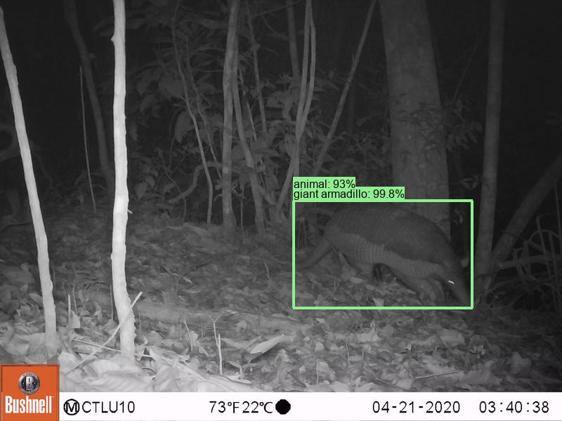
Image credit University of Minnesota, from the Orinoquía Camera Traps dataset.
4 maintainers


Metadata
4 maintainers
Release files for speciesnet 5.0.6
For a detailed explanation of source distributions (sdists) and built distributions (wheels), please see the package formats documentation.
Source distribution (sdist)
| File | Size | Uploaded | |
|---|---|---|---|
| speciesnet-5.0.6.tar.gz | 113.8 kB | Details |
Built distribution (wheel)
| File | Interpreter | ABI | Platform | Reset |
|---|---|---|---|---|
| speciesnet-5.0.6-py3-none-any.whl | Python 3 | none | any | Details |
Total release size: 225.7 kB
Release files / speciesnet-5.0.6.tar.gz
| Download URL | speciesnet-5.0.6.tar.gz |
|---|---|
| Size | 113.8 kB |
| Tags | Source |
|
SHA-256 checksum How to use checksums |
13c3f5f6b413ee7c73548df645d13ebf4ad82a3f924b977ea90a8c8bd56b12b6
|
|
BLAKE2b-256 checksum How to use checksums |
839e2e2876971c0cb49b106abc0ff5e37a9294823b95a5a63b6a8eeda9067844
|
| Upload date | |
|
Uploaded using Trusted Publishing? What is trusted publishing? |
No |
| Uploaded via |
twine/6.1.0 CPython/3.11.11
|
Release files / speciesnet-5.0.6-py3-none-any.whl
| Download URL | speciesnet-5.0.6-py3-none-any.whl |
|---|---|
| Size | 112.0 kB |
| Tags | Python 3 |
|
SHA-256 checksum How to use checksums |
1d7a0ebbf5813de0273bd7702229f90dfd0c671c48d3d819eb9b5332aeab802b
|
|
BLAKE2b-256 checksum How to use checksums |
b7164f26ef5ccec9b914d454414c09966d15005538e5c3930a4fad53991e2820
|
| Upload date | |
|
Uploaded using Trusted Publishing? What is trusted publishing? |
No |
| Uploaded via |
twine/6.1.0 CPython/3.11.11
|














