
SpecPlotter
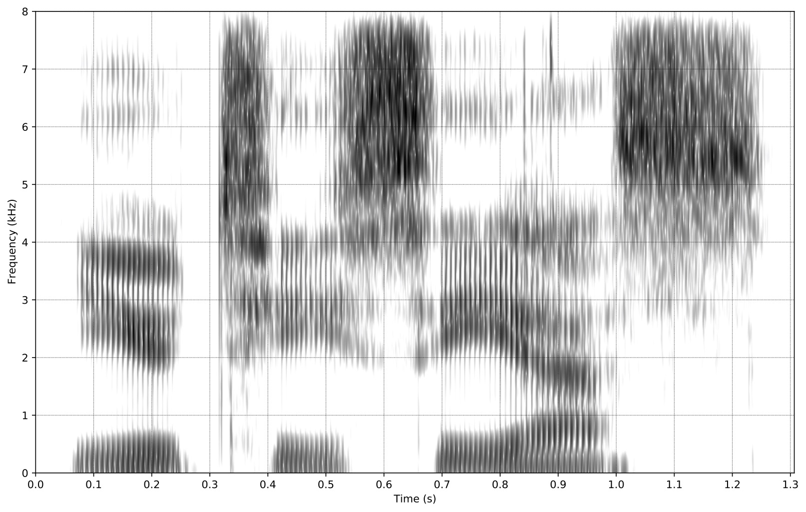
A Python package for creating spectrograms that looks good. Its parameters are carefully tuned by David Harwath to resemble the appearance of physically produced spectrograms, e.g., Kay Sona-Graph.
Installation
pip install specplotter
Quick Start
Command Line Interface
The easiest way to use SpecPlotter is via the command line:
# Basic spectrogram (PNG)
specplotter audio.wav -o output.png

# Basic spectrogram (PDF)
specplotter audio.wav -o output.pdf

# Full analysis with all components
specplotter audio.wav -o output.pdf --zcr --total-energy --lowfreq-energy --waveform

# Narrowband mode
specplotter audio.wav -o output.png --mode narrowband
Python API
from specplotter import SpecPlotter
import librosa

# Load an audio file
signal, sr = librosa.load('audio.wav', sr=16000)

# Create a SpecPlotter instance (default: wideband mode)
plotter = SpecPlotter()

# Plot spectrogram only (default behavior)
plotter.plot_spectrogram(signal)

# Or save to file
plotter.plot_spectrogram(signal, outfile='spectrogram.png')
Usage Examples
Basic Usage
from specplotter import SpecPlotter
import librosa

signal, sr = librosa.load('audio.wav', sr=16000)
plotter = SpecPlotter()

# Default: spectrogram only
plotter.plot_spectrogram(signal)
Wideband vs Narrowband
# Wideband mode (default)
plotter_wide = SpecPlotter(mode='wideband')

# Narrowband mode
plotter_narrow = SpecPlotter(mode='narrowband')

# Plot with different modes
plotter_wide.plot_spectrogram(signal)
plotter_narrow.plot_spectrogram(signal)
Flexible Plotting with Optional Components
# Plot with all components
plotter.plot(
    signal,
    show_zcr=True,
    show_total_energy=True,
    show_lowfreq_energy=True,
    show_waveform=True
)

# Just spectrogram and waveform
plotter.plot(signal, show_waveform=True)

# Spectrogram with zero crossing rate
plotter.plot(signal, show_zcr=True)
Using Custom Axes
import matplotlib.pyplot as plt

# Single axis (spectrogram only)
fig, ax = plt.subplots()
plotter.plot_spectrogram(signal, ax=ax)

# List of axes matching number of plots
fig, axes = plt.subplots(3, 1)  # For zcr, spectrogram, waveform
plotter.plot(
    signal,
    ax=list(axes),
    show_zcr=True,
    show_waveform=True
)

# Full plot with all components
fig, axes = plt.subplots(5, 1)
plotter.plot(
    signal,
    ax=list(axes),
    show_zcr=True,
    show_total_energy=True,
    show_lowfreq_energy=True,
    show_waveform=True
)
Note: When providing a list of axes, they must be in this order:
zcr(ifshow_zcr=True)total_energy(ifshow_total_energy=True)lowfreq_energy(ifshow_lowfreq_energy=True)spectrogram(always included)waveform(ifshow_waveform=True)
Computing Features Without Plotting
# Compute all features
features = plotter.compute_spectrogram(signal)

# Access individual features
processed_signal = features['processed_signal']
spectrogram = features['spectrogram']
zcr = features['zcr']
total_energy = features['total_energy']
lowfreq_energy = features['lowfreq_energy']

# Use features independently
import matplotlib.pyplot as plt
fig, ax = plt.subplots()
plotter._plot_spectrogram_on_axis(spectrogram, len(signal), ax=ax)
Individual Plotting Methods
features = plotter.compute_spectrogram(signal)

# Plot individual components
fig, ax = plt.subplots()
plotter.plot_zcr(features['zcr'], ax=ax)

fig, ax = plt.subplots()
plotter.plot_total_energy(features['total_energy'], ax=ax)

fig, ax = plt.subplots()
plotter.plot_lowfreq_energy(features['lowfreq_energy'], ax=ax)

fig, ax = plt.subplots()
plotter.plot_waveform(features['processed_signal'], ax=ax)
Configuration
Mode Selection
The mode parameter sets default window sizes for wideband or narrowband analysis:
- Wideband (default):
window_size=0.004,window_stride=0.001 - Narrowband:
window_size=0.025,window_stride=0.01
Customizing Parameters
All parameters can be customized when creating a SpecPlotter instance:
plotter = SpecPlotter(
    mode='wideband',              # 'wideband' or 'narrowband'
    sample_rate=16000,            # Sample rate (Hz)
    fnotch=60,                    # Notch filter frequency (Hz)
    notchQ=30,                    # Notch filter Q factor
    preemphasis_coeff=0.97,       # Pre-emphasis coefficient
    window_size=0.004,            # Window size (seconds), optional
    window_stride=0.001,          # Window stride (seconds), optional
    n_fft=1024,                   # Number of FFT points
    window=scipy.signal.windows.hamming,  # Window function
    db_spread=60,                 # Dynamic range (dB)
    db_cutoff=3,                  # Minimum dB value
    fig_height=10,                # Figure height (inches)
    inches_per_sec=10,            # Horizontal scaling
    zcr_smoothing_std=6,          # ZCR smoothing std dev
    zcr_smoothing_size=41,       # ZCR smoothing kernel size
    lowfreq_min=125,              # Low freq energy min (Hz)
    lowfreq_max=750,              # Low freq energy max (Hz)
)
Overriding Mode Defaults
You can override mode defaults by explicitly providing window_size and window_stride:
# Use wideband mode but with custom window settings
plotter = SpecPlotter(
    mode='wideband',
    window_size=0.005,   # Override default
    window_stride=0.002  # Override default
)
Command Line Interface
SpecPlotter includes a command-line interface for quick spectrogram generation.
Basic Usage
specplotter <input_file> -o <output_file>
The output format (PNG or PDF) is automatically determined from the file extension.
Options
Required:
input_file: Path to input WAV file-o, --output: Output file path (must have .png or .pdf extension)
Analysis Mode:
--mode {wideband,narrowband}: Analysis mode (default: wideband)
Additional Plots:
--all: Show all additional plots (zcr, total-energy, lowfreq-energy, waveform)--zcr: Show zero crossing rate plot--total-energy: Show total energy plot--lowfreq-energy: Show low frequency energy plot--waveform: Show waveform plot
Audio Settings:
--sample-rate FLOAT: Sample rate in Hz (default: 16000)
Processing Parameters:
--fnotch FLOAT: Notch filter frequency in Hz (default: 60)--notch-q FLOAT: Notch filter Q factor (default: 30)--db-spread FLOAT: Dynamic range in dB (default: 60)--db-cutoff FLOAT: Minimum dB value to display (default: 3)
Examples
# Basic spectrogram
specplotter audio.wav -o spectrogram.png

# Full analysis (all components)
specplotter audio.wav -o analysis.pdf --all

# Narrowband mode with custom settings
specplotter audio.wav -o output.pdf --mode narrowband --db-spread 80

# Custom sample rate
specplotter audio.wav -o output.png --sample-rate 22050

# European line noise (50 Hz instead of 60 Hz)
specplotter audio.wav -o output.pdf --fnotch 50
Help
For full help and all options:
specplotter --help
API Reference
SpecPlotter.__init__()
Initialize SpecPlotter with configurable parameters. See Configuration section above for all parameters.
compute_spectrogram(signal)
Compute spectrogram and related features.
Parameters:
signal(np.ndarray): Input audio signal
Returns:
dict: Dictionary containing:'processed_signal': Preprocessed signal'spectrogram': Clipped log spectrogram'zcr': Zero crossing rate'total_energy': Total energy envelope'lowfreq_energy': Low frequency energy envelope
plot(signal, ax=None, show_zcr=False, show_total_energy=False, show_lowfreq_energy=False, show_waveform=False, outfile=None, **kwargs)
Plot spectrogram with optional additional features.
Parameters:
signal(np.ndarray): Input audio signalax(Axes or list of Axes, optional): Matplotlib axes to plot onshow_zcr(bool): Whether to show zero crossing rate plotshow_total_energy(bool): Whether to show total energy plotshow_lowfreq_energy(bool): Whether to show low frequency energy plotshow_waveform(bool): Whether to show waveform plotoutfile(str, optional): If provided, save figure to file**kwargs: Additional keyword arguments passed to plotting functions
Returns:
tuple: (figure, axes_dict)
plot_spectrogram(signal, ax=None, outfile=None, **kwargs)
Plot spectrogram only (convenience method).
Parameters:
signal(np.ndarray): Input audio signalax(Axes, optional): Matplotlib axes to plot onoutfile(str, optional): If provided, save figure to file**kwargs: Additional keyword arguments
Returns:
tuple: (figure, axes)
Requirements
- Python >= 3.7
- numpy >= 1.19.0
- scipy >= 1.5.0
- librosa >= 0.8.0
- matplotlib >= 3.3.0
License
MIT License
Versioning
This package uses python-semantic-release for automatic version management based on Conventional Commits.
How it works
The version is automatically determined from your commit messages:
fix:orfix(scope):→ patch version bump (0.0.1 → 0.0.2)feat:orfeat(scope):→ minor version bump (0.0.1 → 0.1.0)feat!:orfix!:orBREAKING CHANGE:→ major version bump (0.0.1 → 1.0.0)
Creating a new release
Simply push commits with conventional commit messages to the main branch:
git commit -m "feat: add new spectrogram visualization feature"
git push origin main
The GitHub Actions workflow will:
- Analyze your commits since the last release
- Determine the appropriate version bump
- Update version numbers in
pyproject.tomland__init__.py - Create a git tag
- Generate/update CHANGELOG.md
- Create a GitHub release
- Build and publish to PyPI (if
PYPI_API_TOKENis configured)
Commit message format
Follow the Conventional Commits specification:
<type>[optional scope]: <description>

[optional body]

[optional footer(s)]
Types:
feat: A new featurefix: A bug fixdocs: Documentation only changesstyle: Code style changes (formatting, etc.)refactor: Code refactoringperf: Performance improvementstest: Adding or updating testschore: Maintenance tasks
Examples:
git commit -m "feat: add support for custom color maps"
git commit -m "fix: correct frequency calculation in spectrogram"
git commit -m "feat!: change API for plot_spectrogram method"
git commit -m "docs: update installation instructions"
Testing
Run tests using pytest:
# Install development dependencies
pip install -e ".[dev]"

# Run all tests
pytest

# Run with verbose output
pytest -v

# Run specific test file
pytest tests/test_specplotter.py
The test suite includes:
- Unit tests for SpecPlotter initialization and configuration
- Tests for spectrogram computation
- Tests for plotting functionality
- Tests for CLI interface
- Tests for error handling
Contributing
Contributions are welcome! Please feel free to submit a Pull Request.
Setting up pre-commit hooks
This project uses pre-commit hooks to ensure code quality. To set them up:
# Install pre-commit
pip install pre-commit

# Install the git hooks
pre-commit install

# Or run manually
pre-commit run --all-files
The pre-commit hooks will automatically:
- Remove trailing whitespace
- Fix end-of-file issues
- Check YAML, JSON, and TOML syntax
- Format code with ruff
- Run ruff linting (with auto-fix)
- Check for merge conflicts
Before submitting
- Run the test suite:
pytest - Run pre-commit hooks:
pre-commit run --all-files - Ensure all tests pass
- Ensure code formatting is correct
1 maintainer

Metadata
1 maintainer
Release files for specplotter 1.1.10
For a detailed explanation of source distributions (sdists) and built distributions (wheels), please see the package formats documentation.
Source distribution (sdist)
| File | Size | Uploaded | |
|---|---|---|---|
| specplotter-1.1.10.tar.gz | 353.7 kB | Details |
Built distribution (wheel)
| File | Interpreter | ABI | Platform | Reset |
|---|---|---|---|---|
| specplotter-1.1.10-py3-none-any.whl | Python 3 | none | any | Details |
Total release size: 367.8 kB
Release files / specplotter-1.1.10.tar.gz
| Download URL | specplotter-1.1.10.tar.gz |
|---|---|
| Size | 353.7 kB |
| Tags | Source |
|
SHA-256 checksum How to use checksums |
e652c6a2948dacdc1be1c2a34b0b61011e20038747d64621e1e67602a9dcc81b
|
|
BLAKE2b-256 checksum How to use checksums |
a4f30cd527061bc58f8d085767dfbebaec859eaa770472d3fd3fa7d5848388d2
|
| Upload date | |
|
Uploaded using Trusted Publishing? What is trusted publishing? |
Yes |
| Uploaded via |
twine/6.1.0 CPython/3.13.7
|
Provenance
Provenance describes where a file came from. On PyPI, provenance is shared via attestations, which provide a verifiable record of the build or publishing details. View details, limitations and caveats.


PyPI Publish Attestation
PyPI verified that this artifact, at this checksum, originated from the publisher listed below.
Signed by GitHub Actions, verified by PyPI on Feb 14, 2026.
Transparency logRelease files / specplotter-1.1.10-py3-none-any.whl
| Download URL | specplotter-1.1.10-py3-none-any.whl |
|---|---|
| Size | 14.0 kB |
| Tags | Python 3 |
|
SHA-256 checksum How to use checksums |
317bec9385c0da9a74ffbd2bbc3942cb552ccece1b551ea2c47f8568ac4c0018
|
|
BLAKE2b-256 checksum How to use checksums |
a2a2baac582cb5b5cf074b4304a0d2019a93d0cdd432df6e5a4b89e9c5f7904a
|
| Upload date | |
|
Uploaded using Trusted Publishing? What is trusted publishing? |
Yes |
| Uploaded via |
twine/6.1.0 CPython/3.13.7
|
Provenance
Provenance describes where a file came from. On PyPI, provenance is shared via attestations, which provide a verifiable record of the build or publishing details. View details, limitations and caveats.
PyPI Publish Attestation
PyPI verified that this artifact, at this checksum, originated from the publisher listed below.
Signed by GitHub Actions, verified by PyPI on Feb 14, 2026.
Transparency log













