Specialized Package for Extracting Image Features for Cardiac Amyloidosis Quantification on SPECT.

Project description
SpectQuant
SpectQuant is a specialized package designed for the feature extraction of special photon emission computer tomography (SPECT) data.
It leverages advanced algorithms known from signal processing and methodologies to standardized results with the potential for scaled data mining.
Special Photon Emission Computer Tomography (SPECT) is an imaging technique that allows for the visualization of functional processes in the body. It involves the detection of gamma rays emitted by a radioactive tracer injected into the patient. The quantitative analysis of SPECT data is crucial for accurate diagnosis and research.
The key steps in the quantitative analysis of SPECT data include:
- Data Processing: Preprocessing the original data by correcting for False Positives, and normalized voxel scores accross images, and image size.
- Feature Extraction: Measuring the concentration of the tracer in different regions of the body.
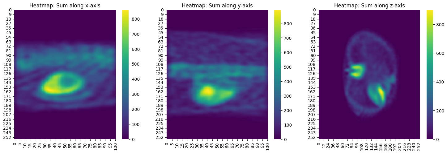
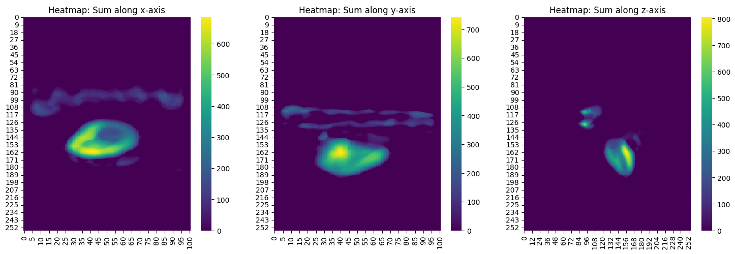
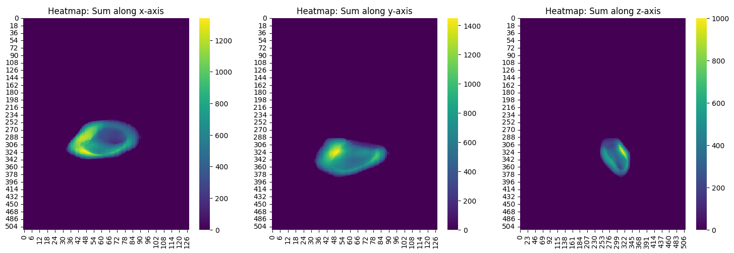
- Visualization: Creating visual representations of the processed data to facilitate interpretation and quick validity assessment.
SUV (Standardized Uptake Value)
For determining the SUV Given a predefined 3D area $A$ (ROI = region of interest) of size $a \cdot a \cdot a$ and a predefined cubic kernel $\kappa$ (3D-window) of size $k \cdot k \cdot k$, the SUV peak is given by the cube (also of size $k \cdot k \cdot k$) at the location where the sum (or mean) of values in $\kappa$ is the highest.
$\forall \alpha_1, \alpha_2, \alpha_3 \in {0, \dots, a}:$ $$ \text{SUV}^{peak} = max\left(\frac{\sum_{\alpha_1, \alpha_2, \alpha_3}^a \kappa}{k \cdot k \cdot k}\right) $$ Essentially, the kernel tries every possible position for $\alpha_{{1,2,3}}$ from $1, \dots, a$ within area $A$ and yields the spot where the kernel $\kappa$ reaches is maximum sum. Then, the arithmetic average is taken from that by dividing by the number of voxels in $\kappa$. This concept alos applies to non-quibic ROIs.
TBR (Target to Blood/Background Ratio)
$$ \text{TBR {peak, mean, mode}} = \frac{\text{SUV {peak, mean, mode}}}{\text{SUV mean vena cava inferior}} $$
Retention Index
$$ \text{SUV retention index} = \left(\frac{\text{SUV peak cardiac}}{\text{SUV peak vertebral}}\right) \times \text{SUV peak paraspinal muscle} $$
Note: see the paper by Rettl et al.
UptakeVol
- Segmentation mask of the given ROI
- Dilation of segmentation mask by 10mm
- Thresholding the entire image: $\forall i \in {1, \dots, x}, j \in {1, \dots, y}, k \in {1, \dots, z}:$ $$ \text{thresholded SPECT} = \begin{cases} 0, & \text{if } \text{SPECT}[i, j, k] < \text{max(SPECT)} \cdot 0.4 \ 1, & \text{otherwise} \end{cases} $$
- If
approach='threshold-bb', the dilated segmentation mask is used to contain the ROI within a 10mm range of the segmentation mask. The dilated segmentation is hence used as a bounding-box.
The 'threshold-bb' is well suited to ensure that no uptake of other structures exceeding the threshold are considered in the volume computation of the ROI:
SeptumVol
- Segmentation masks of the left ventricle (LV) and the right ventricle (RV) are loaded
- Both LV and RV are then enlarged equally in each direction by a dilation algorithm
- Dilated segmentation masks are then cut to avoid false positives in the IVS septum volume due to the dilation.
The cut has been determined by the border voxels' index location of the original/undilated segmentation masks in the follwing ways:
- The dilated LV mask is only cut on the
- x-axis by the highest x-voxel index of the original RV segmentation mask
- The dilated RV mask is cut on
- x-axis: by the lowest x-voxel index of the original LV segmentation mask
- z-axis: by the highest and lowest z-voxel index of the original LV segmentation mask
- The dilated LV mask is only cut on the
$$ {\widehat{RV}} \cup {\widehat{LV}} - {{RV} \cup {\widehat{LV}} + {LV} \cup {\widehat{RV}} } $$
-
${\widehat{RV}}$ = set of voxels of dilated & cut right ventricle
-
${\widehat{LV}}$ = set of voxels of dilated & cut left ventricle
-
${RV}$ = set of voxels of right ventricle
-
${LV}$ = set of voxels of left ventricle
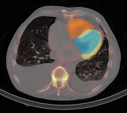
Figure 4: IVS Volume Quantification Process on CT with SPECT overlay showing the tracer uptake.
Release history Release notifications | RSS feed


Download files
Download the file for your platform. If you're not sure which to choose, learn more about installing packages.
Source Distribution
Built Distribution
Filter files by name, interpreter, ABI, and platform.
If you're not sure about the file name format, learn more about wheel file names.
Copy a direct link to the current filters
File details
Details for the file spectquant-0.1.10.tar.gz.
File metadata
- Download URL: spectquant-0.1.10.tar.gz
- Upload date:
- Size: 29.1 kB
- Tags: Source
- Uploaded using Trusted Publishing? No
- Uploaded via: twine/5.1.1 CPython/3.11.4
File hashes
| Algorithm | Hash digest | |
|---|---|---|
| SHA256 |
43b7a2d62cac97402f4990cd363a4d6c6dfe09641befaef799547145b69abfb6
|
|
| MD5 |
6c5fa958fb41c098fd73e3902cbb7df4
|
|
| BLAKE2b-256 |
8458144a51141bbc6f539c24ac36720b5b87447990c085f44e067f4f6b14c906
|
File details
Details for the file spectquant-0.1.10-py3-none-any.whl.
File metadata
- Download URL: spectquant-0.1.10-py3-none-any.whl
- Upload date:
- Size: 30.3 kB
- Tags: Python 3
- Uploaded using Trusted Publishing? No
- Uploaded via: twine/5.1.1 CPython/3.11.4
File hashes
| Algorithm | Hash digest | |
|---|---|---|
| SHA256 |
d585768e54cbf467af49b983f81b3662c74c88234e13b8ef0b73a8c7a99cb7cc
|
|
| MD5 |
3e16c51ac040d584733e3073a905134e
|
|
| BLAKE2b-256 |
4f120d746025a08c8d8ecc620ab74abd1d23f35a5e62108b7a8d5f7ab5d4f96b
|


