
A python library for spectral-zone-level explanations in machine learning models trained on spectral data


Project description

This is the official repository for the spectral-model-explainer (SMX) library, an eXplainable AI tool designed to provide explanations for Machine Learning (ML) models trained on spectral data (e.g., XRF, GRS, Raman, vis-NIR, and related modalities).
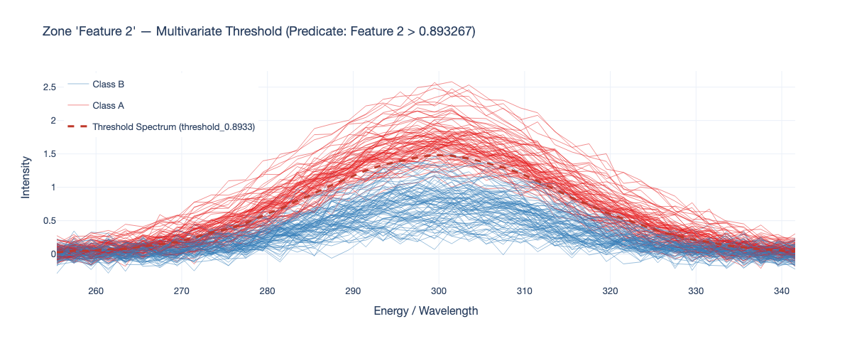
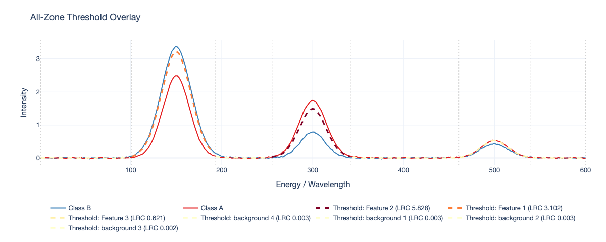
SMX is a post-hoc, global, model-agnostic framework that explains spectral-based ML classifiers directly in terms of expert-informed spectral zones. It aggregates each zone via PCA, formulates quantile-based logical predicates, estimates their relevance through perturbation experiments within stochastic subsamples, and integrates the results into a directed weighted graph whose global structure is summarized by Local Reaching Centrality. A distinctive feature is threshold spectrum reconstruction, which back-projects each predicate's decision boundary into the original spectral domain in natural measurement units, enabling practitioners to visually compare their spectra against the model-related boundaries.
Documentation
Read the latest documentation at https://spectral-model-explainer.readthedocs.io/.
Method Overview in the Library
The high-level workflow is implemented in the SMX pipeline class and can also be executed component-by-component through the public API:
- spectral zone extraction
- zone aggregation (typically PCA-based)
- predicate generation from quantiles
- bagging-based robustness evaluation
- predicate relevance scoring
- directed graph construction
- centrality-based ranking and optional mapping back to natural scale
This implementation allows both:
- end-to-end execution through a single pipeline object
- advanced control through direct use of dedicated classes/functions
Spectral Zone Construction
The method starts by partitioning the spectral axis into zones using extract_spectral_zones. Input spectra are expected as a DataFrame in which columns represent numeric spectral positions (energies, wavelengths, channels, etc.).
How zones must be provided
The cuts argument accepts multiple valid formats:
(start, end)(name, start, end)(name, start, end, group){name, start, end}{name, start, end, group}
Important behavior:
- boundaries are interpreted numerically and inclusively
- if
start > end, the library automatically reorders them - grouped cuts (same
group) are concatenated into one merged zone - non-grouped cuts are kept as independent zones
This flexibility enables both physically meaningful elemental regions and composite regions such as aggregated background segments.
Manual Zone Detection with building_spectral_zones
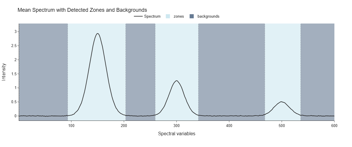
In addition to manually defining spectral zones via the cuts argument, SMX provides building_spectral_zones, a convenience function that automatically detects spectral zones from a single reference spectrum. This is particularly useful when you want to define zones based on the actual peaks and valleys present in your data, rather than predefined boundaries. This function is based on local minima and maxima detection via scipy.signal.argrelmin and scipy.signal.find_peaks, with optional Savitzky-Golay smoothing to enhance robustness against noise. The detected zones are then formatted in the same way as manually defined cuts, allowing seamless integration into the SMX pipeline.
Accordingly, the usage of building_spectral_zones is straightforward and can be directly applied to a representative spectrum or the mean spectrum across samples to identify zones and background segments. The main parameters control the sensitivity of peak detection are:
min_window_length: Minimum length of spectral windows considered for minima extraction, which also controls the minimum width of the resulting zones.prominence: Minimum difference in intensity between a peak and its surrounding baseline for it to be considered a valid peak. Higher values make detection more robust to noise but may miss subtle features.- Optionally, Savitzky-Golay smoothing can be applied before peak detection (
svg_smooth=True) to further improve robustness in noisy spectra.
As an example:
from smx.zones import building_spectral_zones

# spectrum: DataFrame, Series, or array with spectral data
spectral_cuts = building_spectral_zones(
    spectrum,                # Reference spectrum for zone detection
    min_window_length=7,      # Window for local minima detection (order parameter for argrelmin)
    prominence=0.3,          # Minimum prominence for peak detection
    svg_smooth=False,        # Apply Savitzky-Golay smoothing before detection
    svg_window_length=7,      # SG window length (if svg_smooth=True)
    svg_polyorder=3,         # SG polynomial order (if svg_smooth=True)
    svg_deriv=0,             # SG derivative order (0=smoothing only, 1=first derivative, etc.)
    ploting=True,            # Generate visualization with detected zones
    output_path="detected_zones.png",  # Save plot to file
)
Returns: A list of spectral cuts in the format [(name, start, end), ...], where zones are automatically labeled as zone1, zone2, ... and background segments as background1, background2, ...
The function automatically identifies local minima (valleys) and maxima (peaks) in the spectrum, then constructs zones bounded by consecutive minima, alternating between spectral features (zones) and inter-feature regions (background).
Predicate Construction from Zone Scores
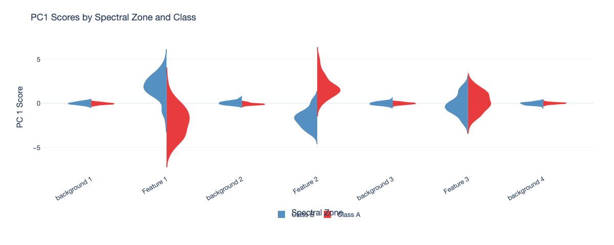
After extraction, each zone is transformed into one scalar score per sample (default strategy: PC1 score via ZoneAggregator(method="pca")). These zone-level summaries are the basis for predicate generation.
PredicateGenerator creates binary threshold predicates from a user-defined set of quantiles. For each zone and each quantile value q, two complementary predicates are produced:
zone <= threshold(q)zone > threshold(q)
Therefore, if k quantiles are provided, the initial candidate set is 2k predicates per zone (before duplicate removal). Duplicate rules are automatically removed when quantiles collapse to identical threshold values.
Bagging and Robustness Hyperparameters
SMX estimates predicate robustness through repeated bagging cycles. In the high-level pipeline, this is controlled primarily by:
n_bags: number of bags generated per repetition (seed)n_repetitions: number of independent repetitions (seed loop)n_samples_fraction: fraction of samples drawn in each bagquantiles: quantile grid that defines predicate thresholds
Operationally:
- each repetition creates a new random context for bag generation
- each bag evaluates which predicates are sufficiently supported by sampled data
- predicates with very low support in a bag are discarded for that bag
- final rankings are aggregated across valid repetitions to reduce seed sensitivity
This design makes the explanation less dependent on a single random split and more representative of stable decision behavior.
Predicate Relevance and Graph Construction
Within each bag, predicates are ranked by an importance metric based on perturbation experiments:
- perturbation-based relevance (
PerturbationMetric), using a fitted estimator
PredicateGraphBuilder then constructs a directed graph from ranked predicates:
- consecutive predicates in a ranking induce directed edges
- edge weights are accumulated across bags
- terminal class nodes are linked from last predicates in each path
- bidirectional conflicts are resolved by keeping the stronger direction (ties are randomized)
- edge weighting can incorporate zone-level explained variance from PCA (
var_exp=True), which constrains the graph structure to reflect both predictive relevance and variance importance of zones
Finally, the graph is summarized through Local Reaching Centrality (LRC), producing a ranked list of influential predicates/zones. Accordngly, the final output is a DataFrame with predicates ranked by their LRC scores, along with their corresponding natural-scale thresholds and zone information. This allows practitioners to identify which spectral zones and thresholds are most influential in the model's decision-making process, providing insights into the underlying spectral features driving predictions. Beyond identifying relevant zones, the predicate's threshold values themselves live in PCA space and are back-projected to the original domain as per-zone multivariate thresholds that can be overlaid on measured spectra, translating an abstract condition into a physically readable boundary. Thus, SMX goes beyond numerical importances by delivering condition-aware, subset-aware explanations that support validation, hypothesis generation, and more actionable domain conclusions.
Model Compatibility Note
At the current stage, SMX is primarily designed for use with scikit-learn-style estimators. In practical terms, this means that when the perturbation-based relevance strategy is employed, the estimator passed to the pipeline is expected to be already fitted and to expose the standard prediction interface required by the selected perturbation metric.
More specifically, the minimum requirement is a valid predict method. In addition, some perturbation metrics require richer interfaces: probability_shift requires predict_proba, while decision_function_shift requires decision_function. Consequently, any model class that follows this contract can be integrated in a technically consistent manner, independently of the specific learning algorithm (for example, SVMs, tree ensembles, linear models, and related scikit-learn-compatible estimators).
Ongoing development is focused on extending this compatibility layer beyond the current scikit-learn-centric workflow, with the objective of supporting additional model ecosystems and API styles in Python while preserving methodological consistency and interpretability guarantees.
Installation and Optional Plotting Dependency
SMX is intentionally distributed with a lightweight core dependency set, where visualization is treated as an optional capability rather than a mandatory runtime requirement. This design ensures that users interested exclusively in methodological analysis (zone extraction, predicate construction, bagging, graph construction, and centrality-based ranking) can install and execute the framework without incurring additional graphical dependencies.
Base installation:
pip install spectral-model-explainer
Installation with plotting support:
pip install "spectral-model-explainer[plotting]"
In practical terms, the plotting extra enables functions that generate interactive visual outputs (for example, threshold-spectrum overlays used to inspect reconstructed multivariate decision boundaries in the natural spectral domain). The analytical SMX pipeline remains fully functional without this extra.
If plotting routines are invoked in an environment where the plotting extra has not been installed, SMX raises an explicit import-related error with installation guidance. This behavior is intentional: it preserves minimal installation overhead for non-visual workflows while providing clear and immediate feedback when visualization features are requested.
Easy Usage
import pandas as pd
from sklearn.svm import SVC
from smx import SMX

X_cal_prep # preprocessed calibration spectra (DataFrame)
X_cal_natural # original calibration spectra before preprocessing (DataFrame)
y_cal_labels # class labels for calibration samples (Series)

spectral_cuts = [...]  # Define or extract spectral zones (see building_spectral_zones)

model = SVC(kernel="rbf", probability=True, random_state=42)
model.fit(X_cal_prep, y_cal_labels)

# Example: probability of the first class as continuous output

smx = SMX(
spectral_cuts=spectral_cuts, # list of spectral zones defined by cuts (start, end) or (name, start, end) or (name, start, end, group)
quantiles=[0.2, 0.4, 0.6, 0.8], # quantiles for predicate generation (each quantile produces two predicates: <= and >)
n_repetitions=4, # number of independent repetitions
n_bags=10,
n_samples_fraction=0.8,
estimator=model,
perturbation_metric="probability_shift" # metric for evaluating predicate relevance (supports "probability_shift", "decision_function_shift", among others)
)

smx.fit(X_cal_prep = X_cal_prep, # preprocessed calibration spectra for predicate evaluation
        y_pred_cal = model.predict_proba(X_cal_prep)[:, 0],  # predicted probabilities for classes (it can be either 0 or 1) for building the terminal nodes
        X_cal_natural = X_cal_natural # natural-scale calibration spectra mapped back to the original domain
        )

# Main result (ranked predicates with natural-scale thresholds)
results = smx.lrc_natural_
print(results.head())

# Optional: evaluate explanation faithfulness on a held-out set
faithfulness = smx.evaluate_faithfulness(
    X_test_prep,
    ranking="unique",
    masking_strategy="zero",
    output_path="faithfulness_curve.html",
)
print(faithfulness["level"], faithfulness["auc"], faithfulness.get("plot_path"))
Plotting Gallery
SMX ships seven interactive Plotly visualizations that turn LRC results into
immediately readable explanations. All figures accept a unified SMXTheme
for consistent styling and support both .html (interactive) and
.png / .svg / .pdf (static, via kaleido) output formats.
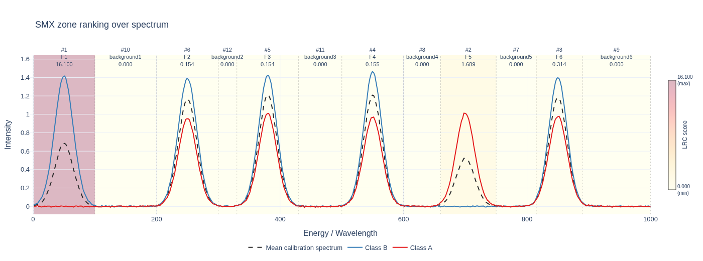 Zone Ranking |
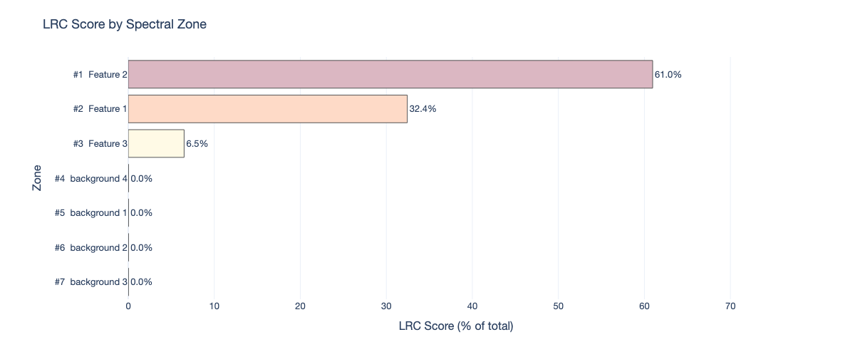 Zone Importance |
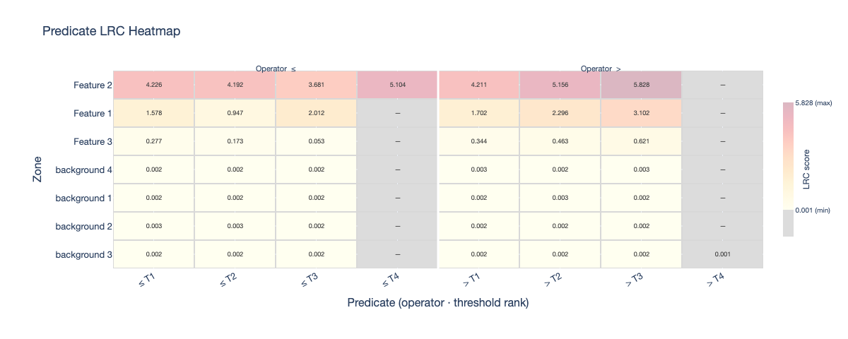 Predicate Heatmap |
 Threshold Spectrum |
 All-Zone Threshold Overlay |
 Zone Higher Variance Score |
→ See the full Plotting Gallery for usage examples and parameter reference.
Plotting Helpers
SMX includes Plotly-based visualization helpers for common explanation views.
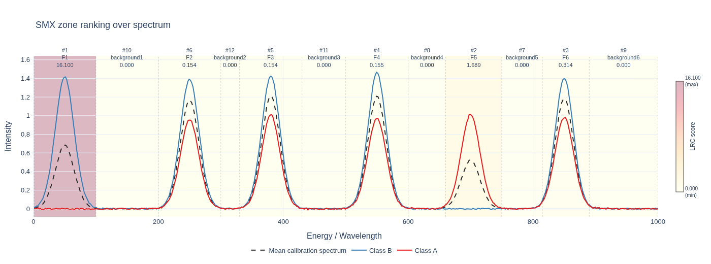
Zone Ranking Over Spectrum
After fitting an SMX explainer, you can export the ranked spectral zones over
the reference spectrum. The output format is inferred from the file extension —
use .html for an interactive figure or .png / .svg / .pdf for a static
image (requires pip install kaleido):
from smx import SMX

explainer=SMX(...) # SMX instance after fitting (see easy usage for example)

explainer.fit(X_cal_prep, y_pred_cal, X_cal_natural=X_cal_raw)

# Interactive HTML
explainer.plot_zone_ranking_over_spectrum("zone_ranking.html", ranking="unique")

# Static PNG (requires kaleido)
explainer.plot_zone_ranking_over_spectrum(
    "zone_ranking.png",
    ranking="unique",
    X_natural=X_cal_raw,
    y_labels=y_cal,
    width=1400,
    height=520,
)
You can also call the standalone plotting function:
from smx import plot_zone_ranking_over_spectrum

plot_zone_ranking_over_spectrum(
    zone_ranking_df=explainer.lrc_summed_unique_,
    spectral_cuts=spectral_cuts,
    reference_spectrum=explainer.zones_natural_,
    output_path="zone_ranking.png",   # or .html
    class_spectra={"A": X_cal[y_cal == "A"], "B": X_cal[y_cal == "B"]},
)
Faithfulness Evaluation
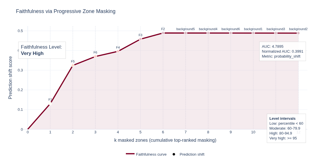
SMX provides a built-in progressive masking protocol to assess how faithfully an explanation reflects the model's actual decision behaviour. Given a held-out evaluation set, the method works as follows:
- Zones are masked one at a time, in order of decreasing LRC score
- The classifier's prediction is recomputed after each masking step
- A prediction-shift curve is built by accumulating the changes in the model's output as more zones are removed
The result is summarised by the Area Under the Curve (AUC) of this masking curve. A high AUC indicates that the top-ranked zones carry most of the model's discriminative power — i.e. the explanation is faithful. A low AUC (close to random ordering) suggests the ranking does not reflect the model's actual decision logic.
The output of evaluate_faithfulness includes:
-
auc— trapezoidal AUC of the masking curve. Raw AUC values are bounded by the total number of zones and the model's baseline accuracy; they are normalised to the [0, 1] interval by dividing by the maximum achievable AUC (i.e. the AUC of a perfectly ordered ranking that masks the least-informative zones first). -
level— a categorical quality label assigned as follows:Level Condition very high null_percentile ≥ 95high null_percentile ≥ 90moderate null_percentile ≥ 75low null_percentile ≥ 50very low null_percentile < 50 -
null_percentile— percentile of the true AUC against a null distribution built by computing the AUC for a large number of random zone orderings (default: 500 permutations). A percentile close to 100 means the LRC-based ranking is far better than random; a percentile near 50 means the ranking carries no more information than chance. -
curve_df— a DataFrame with columnsk,masked_zone,masked_zones, andscoredescribing the curve point at each masking step -
plot_path— path to a saved interactive Plotly HTML figure (whenoutput_pathis provided) -
null_distribution— list of AUC values from the null (random) permutations, useful for diagnostic histograms -
k— number of top zones at which the maximum drop in prediction score is observed
Interpretation guide for the masking curve:
- Steep early drop (top-left of curve is high) — the first few zones dominate the prediction, confirming that the LRC ranking captures the core decision boundary
- Gradual decline — predictive power is distributed across many zones; the model relies on a broad spectral signature rather than a few sharp features
- Flat curve — masking has little effect regardless of zone order, indicating either a weak classifier or a ranking that is misaligned with decision behaviour
The curve is visualised via plot_faithfulness_curve, which draws the prediction-shift curve with a shaded AUC region and annotates the summary statistics. Pass show_percentile=True to overlay the null-distribution percentile band on the figure.
# After fitting an SMX explainer
faithfulness = smx.evaluate_faithfulness(
    X_test_prep,
    ranking="unique",
    masking_strategy="zero",
    metric="auto", # automatically selects "probability_shift", "decision_function_shift", or "mean_abs_diff" based on the estimator's available methods
    output_path="faithfulness_curve.html",
)
print(f"AUC: {faithfulness['auc']:.4f} | Level: {faithfulness['level']} | "
      f"Null percentile: {faithfulness['null_percentile']:.1f}%")
For a complete, executable walkthrough with synthetic data and visualization outputs, see the quickstart notebook:
Citation
If you use SMX in your research, please cite:
@misc{ribeiro2026spectralmodelexplainer,
      title={Spectral Model eXplainer: a chemically-grounded explainability framework for spectral-based machine learning models},
      author={Jose Vinicius Ribeiro and Rafael Figueira Goncalves and Fabio Luiz Melquiades and Sylvio Barbon Junior},
      year={2026},
      eprint={2605.02684},
      archivePrefix={arXiv},
      primaryClass={cs.LG},
      url={https://arxiv.org/abs/2605.02684},
}
License
This project is licensed under the MIT License. See the LICENSE file for details.
Release history Release notifications | RSS feed


Download files
Download the file for your platform. If you're not sure which to choose, learn more about installing packages.
Source Distribution
Built Distribution
Filter files by name, interpreter, ABI, and platform.
If you're not sure about the file name format, learn more about wheel file names.
Copy a direct link to the current filters
File details
Details for the file spectral_model_explainer-0.1.10.tar.gz.
File metadata
- Download URL: spectral_model_explainer-0.1.10.tar.gz
- Upload date:
- Size: 67.6 kB
- Tags: Source
- Uploaded using Trusted Publishing? No
- Uploaded via: poetry/2.4.0 CPython/3.11.15 Linux/6.17.0-1013-azure
File hashes
| Algorithm | Hash digest | |
|---|---|---|
| SHA256 |
f5fca65649d2606bd0585a2520ab9d917788a0aaa6c79fdd62a994108e252d1e
|
|
| MD5 |
7c3ffa788a61354b3d98f225748a7959
|
|
| BLAKE2b-256 |
295665fc991d0c65a72cc4a4591e6c998a026e99f47d237e5e52c51f946ab518
|
File details
Details for the file spectral_model_explainer-0.1.10-py3-none-any.whl.
File metadata
- Download URL: spectral_model_explainer-0.1.10-py3-none-any.whl
- Upload date:
- Size: 74.1 kB
- Tags: Python 3
- Uploaded using Trusted Publishing? No
- Uploaded via: poetry/2.4.0 CPython/3.11.15 Linux/6.17.0-1013-azure
File hashes
| Algorithm | Hash digest | |
|---|---|---|
| SHA256 |
bc40f3bebfcb26d0f45ccb83ab7d21a98fda329e15f7f16cbd5265c6467b0da3
|
|
| MD5 |
9a2e87205bec2437ef2ecaf399172159
|
|
| BLAKE2b-256 |
f397b1d0f14685eca3e654d1024f22b4d304119c0cf8b96e229165ebbd8889a2
|






