
spey-hs3: HS3 Statistical Models in Spey










spey-hs3 is a Spey plug-in that enables statistical inference on models described in the
HEP Statistics Serialization Standard (HS3) JSON format via the
pyhs3 backend. It exposes the full Spey API
(CLs values, upper limits, likelihood evaluations, etc.) for any HS3-compatible
workspace.
Related resources
Installation
pip install spey spey-hs3
The plug-in registers itself automatically as the hs3 backend and is
immediately available via spey.get_backend("hs3").
Overview
A typical HS3 workspace is a JSON document that encodes one or more
histfactory_dist distributions (channels), observed data, nuisance
parameters, and their domains. spey-hs3 reads this document, optionally
injects a new signal sample into the relevant channels, compiles the pyhs3
model, and wraps it in a Spey StatisticalModel so that all standard
hypothesis-testing routines work out of the box.
The signal yields are not part of the HS3 workspace file itself; they are supplied separately as a nested Python dictionary and injected at construction time. This keeps the background model and signal hypothesis cleanly separated.
Quick Start
1. Define the workspace and signal
The example below constructs a minimal two-bin HS3 workspace by hand. In practice you would load a workspace from a JSON file produced by a statistics framework (e.g. RooFit or pyhf).
import spey
import numpy as np

# Minimal two-bin HS3 workspace (background-only model)
simple_hs3 = {
    "metadata": {"hs3_version": "0.2"},
    "distributions": [
        {
            "name": "channel",
            "type": "histfactory_dist",
            "axes": [{"name": "obs", "edges": [0.0, 1.0, 2.0]}],
            "samples": [
                {
                    "name": "bkg",
                    "data": {"contents": [40.0, 60.0], "errors": [0.0, 0.0]},
                    "modifiers": [
                        {
                            "name": "mu_bkg",
                            "type": "normfactor",
                            "parameter": "mu_bkg",
                        },
                        {
                            "name": "bkg_sys",
                            "type": "normsys",
                            "parameter": "alpha_bkg",
                            "data": {"lo": 0.90, "hi": 1.10},
                        },
                    ],
                }
            ],
        }
    ],
    "parameter_points": [
        {
            "name": "nominal",
            "parameters": [
                {"name": "mu",       "value": 1.0},
                {"name": "mu_bkg",   "value": 1.0, "const": True},
                {"name": "alpha_bkg","value": 0.0},
            ],
        }
    ],
    "domains": [
        {
            "name": "model_domain",
            "type": "product_domain",
            "axes": [
                {"name": "mu",       "min": -5.0, "max": 10.0},
                {"name": "mu_bkg",   "min":  0.0, "max":  3.0},
                {"name": "alpha_bkg","min": -5.0, "max":  5.0},
            ],
        }
    ],
    "data": [
        {
            "name": "observed",
            "type": "binned",
            "contents": [53, 57],
            "axes": [{"name": "obs", "edges": [0.0, 1.0, 2.0]}],
        }
    ],
    "likelihoods": [
        {"name": "L", "distributions": ["channel"], "data": ["observed"]}
    ],
    "analyses": [
        {
            "name": "demo",
            "likelihood": "L",
            "domains": ["model_domain"],
            "parameters_of_interest": ["mu"],
            "init": "nominal",
        }
    ],
}

# Signal: 5 events per bin injected as a new sample in "channel"
simple_signal = {"channel": {"signal": [5.0, 5.0]}}
The workspace defines a single channel (channel) with:
- a background sample (
bkg) with nominal yields of 40 and 60 events across two bins; - a normalisation modifier
mu_bkg(fixed to 1 at nominal) and a correlated shape/normalisation systematicalpha_bkg(±10 %); - observed data of 53 and 57 events;
- the signal-strength parameter of interest
muwith domain [−5, 10].
The signal dictionary adds 5 events per bin to the channel distribution.
This sample is automatically given a normfactor modifier tied to mu so
that it scales linearly with the signal strength.
2. Construct the statistical model
HS3 = spey.get_backend("hs3")

simple_model = HS3(
    hs3_dict=simple_hs3,
    signal_yields=simple_signal,
    mode="FAST_COMPILE",
)
mode="FAST_COMPILE" uses PyTensor's fast compilation path, which reduces
start-up time at the cost of some runtime optimisation — suitable for
interactive work. Switch to "FAST_RUN" for computationally intensive scans.
3. Compute CLs at the nominal signal strength
With the model built, calling exclusion_confidence_level() runs the
profile-likelihood ratio test for the hypothesis mu = 1:
cls_s_obs = simple_model.exclusion_confidence_level(
    expected=spey.ExpectationType.observed
)
cls_s_exp = simple_model.exclusion_confidence_level(
    expected=spey.ExpectationType.apriori
)

print(f"Observed CLs (mu=1) = {cls_s_obs[0]:.4f}")
print(f"Expected CLs (mu=1) = {cls_s_exp[2]:.4f}")
# Observed CLs (mu=1) = 0.2361
# Expected CLs (mu=1) = 0.5299
exclusion_confidence_level returns a list of five values corresponding to
the [−2σ, −1σ, median, +1σ, +2σ] quantiles of the expected distribution.
cls_s_obs[0] is the single observed value; cls_s_exp[2] is the median
expected value (under the background-only hypothesis).
Because the observed data are close to the background expectation of 100 events
and the signal contributes only 10 events in total, the model has low
sensitivity and does not exclude mu = 1.
4. Compute the 95 % CL upper limit on the signal strength
The upper limit on mu is the value at which the CLs p-value equals 0.05:
mu_ul_obs = simple_model.poi_upper_limit(
    expected=spey.ExpectationType.observed,
    confidence_level=0.95,
)
mu_ul_exp = simple_model.poi_upper_limit(
    expected=spey.ExpectationType.apriori,
    confidence_level=0.95,
)

print(f"Observed  mu_UL (95% CL) = {mu_ul_obs:.4f}")
print(f"Expected  mu_UL (95% CL) = {mu_ul_exp:.4f}")
# Observed  mu_UL (95% CL) = 4.0300
# Expected  mu_UL (95% CL) = 2.7343
The observed upper limit (~4.0) is larger than the expected (~2.7) because the data are slightly above the background prediction, reducing the sensitivity relative to the expectation.
5. CLs scan and Brazilian plot
To visualise the full CLs curve and its expected uncertainty band, scan mu
over a range of values and retrieve both the observed and expected (±1σ, ±2σ)
CLs values:
import matplotlib.pyplot as plt

mu_scan = np.linspace(2.5, 6.0, 50)

# Observed CLs at each mu
cls_obs = np.array(
    [
        simple_model.exclusion_confidence_level(
            poi_test=mu,
            expected=spey.ExpectationType.observed,
        )[0]
        for mu in mu_scan
    ]
)

# Expected CLs (all five quantiles) at each mu
cls_exp = np.array(
    [
        simple_model.exclusion_confidence_level(
            poi_test=mu,
            expected=spey.ExpectationType.aposteriori,
        )
        for mu in mu_scan
    ]
)

# Upper limits
mu_ul_obs = simple_model.poi_upper_limit(
    expected=spey.ExpectationType.observed,
    confidence_level=0.95,
)
mu_ul_exp = simple_model.poi_upper_limit(
    expected=spey.ExpectationType.aposteriori,
    confidence_level=0.95,
)

fig, ax = plt.subplots()

# Observed CLs curve
ax.plot(mu_scan, cls_obs, "-", color="steelblue", lw=2, label="Observed")

# Expected median and uncertainty bands
ax.plot(
    mu_scan, cls_exp[:, 2],
    "--", color="red", lw=2, label=r"Expected $\pm1\sigma,\,\pm2\sigma$",
)
ax.fill_between(mu_scan, cls_exp[:, 1], cls_exp[:, 3], color="tab:green", alpha=0.5, lw=0)
ax.fill_between(mu_scan, cls_exp[:, 0], cls_exp[:, 4], color="yellow",    alpha=0.2, lw=0)

# 95 % CL threshold and upper-limit markers
ax.axhline(0.95, ls="--", color="firebrick", lw=2, label=r"95\% CL threshold")
ax.axvline(
    mu_ul_obs, ls=":", color="gray", lw=2,
    label=rf"$\mu^{{\rm obs}}_{{\rm UL}}$ = {mu_ul_obs:.2f}",
)
ax.axvline(
    mu_ul_exp, ls=":", color="purple", lw=2,
    label=rf"$\mu^{{\rm exp}}_{{\rm UL}}$ = {mu_ul_exp:.2f}",
)

ax.set_xlabel(r"Signal strength $\mu$")
ax.set_ylabel(r"$\mathrm{CL}_s$")
ax.legend(fontsize=13)
plt.tight_layout()
plt.show()
The resulting plot is shown below.
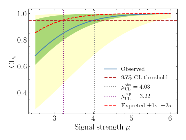
The plot displays the CLs value as a function of the signal-strength parameter
mu:
- Blue solid line — observed CLs, computed from the actual data in the workspace.
- Red dashed curve — median expected CLs under the background-only hypothesis.
- Green / yellow bands — ±1σ and ±2σ expected uncertainty bands (the "Brazilian flag" pattern characteristic of CLs plots in HEP).
- Red dashed horizontal line — the 95 % CL threshold (CLs = 0.95); signal strengths above the intersection with the CLs curve are excluded.
- Gray / purple dotted vertical lines — observed and expected 95 % CL
upper limits on
mu, both near 4.0 for this model. The observed limit is slightly higher than the expected limit because the data lie a little above the background prediction, which reduces the discriminating power.
Loading a workspace from a file
In practice, HS3 workspaces are serialised as JSON files. Load them with the
standard json module and pass the resulting dictionary to HS3Interface:
import json
import spey

with open("workspace.json") as f:
    hs3_dict = json.load(f)

signal = {"model_SR": {"Signal": [3.0, 5.0, 2.0]}}

stat_model = spey.get_backend("hs3")(
    hs3_dict=hs3_dict,
    signal_yields=signal,
    analysis_name="myAnalysis",   # optional; defaults to first analysis
)

stat_model.exclusion_confidence_level()
WorkspaceInterpreter
WorkspaceInterpreter is a lightweight helper for inspecting HS3 workspaces
and preparing signal injections without compiling the pyhs3 model. It is
analogous to the pyhf WorkspaceInterpreter but operates directly on the raw
JSON dictionary.
from spey_hs3 import WorkspaceInterpreter

interp = WorkspaceInterpreter(hs3_dict)
interp.summary()
============================================================
HS3 Workspace Summary
  hs3_version : 0.2
  analyses              : 1
  likelihoods           : 1
  histfactory dists     : 1
  data entries          : 1

Analysis : demo
  POIs      : ['mu']
  Likelihood: L
  Distributions (1):
       1.      channel  (2 bins)  obs=2
============================================================
Inspection properties
| Property | Description |
|---|---|
interp.distributions |
Names of all histfactory_dist distributions |
interp.analyses |
Names of all analyses |
interp.poi_names |
POIs per analysis: {analysis: [poi, ...]} |
interp.samples |
Sample names per distribution |
interp.modifier_types |
Modifier types per sample per distribution |
interp.bin_map |
Number of bins per distribution |
interp.expected_background_yields |
Total background per bin per distribution |
interp.observed_data |
Observed data per distribution |
interp.parameters |
Parameter metadata from the nominal parameter point |
Signal injection
Use inject_signal to add a single signal sample to one distribution, or
inject_signals to inject into multiple distributions at once. After
injection, use the patch property to obtain the modified workspace dictionary:
# Single distribution
interp.inject_signal("channel", "signal", [5.0, 5.0])

# Multiple distributions at once
interp.inject_signals({
    "model_SR_0j": {"Signal": [3.0, 5.0, 2.0]},
    "model_SR_1j": {"Signal": {"contents": [1.0, 2.0], "errors": [0.1, 0.2]}},
})

# Retrieve patched workspace and pass to HS3Interface
stat_model = spey.get_backend("hs3")(hs3_dict=interp.patch)
The injected sample automatically receives a normfactor modifier tied to the
analysis POI, so that mu scales the signal yields when the model is
evaluated.
Other operations
# Remove a distribution from the workspace
interp.remove_distribution("model_CR")

# Reset all injected signals and removal requests
interp.reset_signal()

# Save the patched workspace to disk
interp.save_patch("patched_workspace.json")
API reference
Full documentation (including the complete API reference and advanced usage examples) is available at spey-hs3.readthedocs.io.
For questions or issues please open a ticket on GitHub.
1 maintainer

Metadata
1 maintainer
Release files for spey-hs3 0.0.3
For a detailed explanation of source distributions (sdists) and built distributions (wheels), please see the package formats documentation.
Source distribution (sdist)
| File | Size | Uploaded | |
|---|---|---|---|
| spey_hs3-0.0.3.tar.gz | 37.9 kB | Details |
Built distribution (wheel)
| File | Interpreter | ABI | Platform | Reset |
|---|---|---|---|---|
| spey_hs3-0.0.3-py3-none-any.whl | Python 3 | none | any | Details |
Total release size: 67.0 kB
Release files / spey_hs3-0.0.3.tar.gz
| Download URL | spey_hs3-0.0.3.tar.gz |
|---|---|
| Size | 37.9 kB |
| Tags | Source |
|
SHA-256 checksum How to use checksums |
e03a46536fa9759cc4cb6d5abed612e112a3b0b0605db645419b8058f88145ae
|
|
BLAKE2b-256 checksum How to use checksums |
42ae7902d4ade3b2658288d8c36c1cdab44f22881eb09f1298ce7b12adb83c2d
|
| Upload date | |
|
Uploaded using Trusted Publishing? What is trusted publishing? |
No |
| Uploaded via |
twine/6.1.0 CPython/3.13.7
|
Release files / spey_hs3-0.0.3-py3-none-any.whl
| Download URL | spey_hs3-0.0.3-py3-none-any.whl |
|---|---|
| Size | 29.1 kB |
| Tags | Python 3 |
|
SHA-256 checksum How to use checksums |
5725ea548837b8ec112707266c629feaf2324c5d9241bbf314d04947a8c4986b
|
|
BLAKE2b-256 checksum How to use checksums |
8a3091f6e95c45a846d27670f1451dfb58d7cb7cf57c0e7b1ca8ba5df60b4ad9
|
| Upload date | |
|
Uploaded using Trusted Publishing? What is trusted publishing? |
No |
| Uploaded via |
twine/6.1.0 CPython/3.13.7
|














