Smooth inference for reinterpretation studies

Project description
Spey: smooth inference for reinterpretation studies


Outline
Installation
Spey can be found in PyPi library and can be downloaded using
pip install spey
If you like to use a specific branch, you can either use make install or pip install -e . after cloning the repository or use the following command:
python -m pip install --upgrade "git+https://github.com/SpeysideHEP/spey"
Note that main branch may not be the stable version.
To install a specific branch with pip, use the following command:
python -m pip install git+https://github.com/SpeysideHEP/spey@<BRANCH>
Please be aware that non-released branches are not stable.
What is Spey?
Spey is a plug-in-based statistics framework designed to be fully backend-agnostic, providing a unified environment where all likelihood prescriptions can be compiled and accessed in one place. This enables users to flexibly combine diverse statistical models and analyse them through a single, coherent interface. In line with the FAIR principles, ensuring that models are findable, accessible, interoperable, and reusable, Spey adopts a modular plug-in system allowing developers to contribute statistical model prescriptions in a transparent and future-proof manner, ensuring compatibility with both current and evolving standards.
Finally, the name "Spey" originally comes from the Spey River, a river in the mid-Highlands of Scotland. The area "Speyside" is famous for its smooth whisky.
What a plugin provides
A quick intro on the terminology of spey plugins in this section:
- A plugin is an external Python package that provides additional statistical model prescriptions to spey.
- Each plugin may provide one (or more) statistical model prescriptions that are accessible directly through Spey.
- Depending on the scope of the plugin, you may wish to provide additional (custom) operations and differentiability through various autodif packages such as
autogradorjax. As long as they are implemented through a set of predefined function names spey can automatically detect and use them within the interface.
Currently available plug-ins
| Accessor | Description |
|---|---|
"default.uncorrelated_background" |
Constructs uncorrelated multi-bin statistical model. |
"default.correlated_background" |
Constructs correlated multi-bin statistical model with Gaussian nuisances. |
"default.third_moment_expansion" |
Implements the skewness of the likelihood by using third moments. |
"default.effective_sigma" |
Implements the skewness of the likelihood by using asymmetric uncertainties. |
"default.poisson" |
Implements simple Poisson-based likelihood without uncertainties. |
"default.normal" |
Implements Normal distribution. |
"default.multivariate_normal" |
Implements Multivariate normal distribution. |
"pyhf.uncorrelated_background" |
Uses uncorrelated background functionality of pyhf (see spey-phyf plugin). |
"pyhf" |
Uses generic likelihood structure of pyhf (see spey-phyf plugin) |
For details on all the backends, see the Plug-ins section of the documentation.
Quick Start
First one needs to choose which backend to work with. By default, spey is shipped with various types of
likelihood prescriptions which can be checked via AvailableBackends function
import spey
print(spey.AvailableBackends())
# ['default.correlated_background',
#  'default.effective_sigma',
#  'default.third_moment_expansion',
#  'default.uncorrelated_background']
Using 'default.uncorrelated_background' one can simply create single or multi-bin
statistical models:
pdf_wrapper = spey.get_backend('default.uncorrelated_background')

data = [1]
signal_yields = [0.5]
background_yields = [2.0]
background_unc = [1.1]

stat_model = pdf_wrapper(
    signal_yields=signal_yields,
    background_yields=background_yields,
    data=data,
    absolute_uncertainties=background_unc,
    analysis="single_bin",
    xsection=0.123,
)
where data indicates the observed events, signal_yields and background_yields represents
yields for signal and background samples and background_unc shows the absolute uncertainties on
the background events i.e. $2.0\pm1.1$ in this particular case. Note that we also introduced
analysis and xsection information which are optional where the analysis indicates a unique
identifier for the statistical model, and xsection is the cross-section value of the signal, which is
only used for the computation of the excluded cross-section value.
During the computation of any probability distribution, Spey relies on the so-called "expectation type".
This can be set via spey.ExpectationType which includes three different expectation modes.
-
spey.ExpectationType.observed: Indicates that the computation of the log-probability will be achieved by fitting the statistical model on the experimental data. For the exclusion limit computation, this will tell the package to compute observed ${\rm CL}_s$ values.spey.ExpectationType.observedhas been set as default throughout the package. -
spey.ExpectationType.aposteriori: This command will result in the same log-probability computation asspey.ExpectationType.observed. However, the expected exclusion limit will be computed by centralizing the statistical model on the background and checking $\pm1\sigma$ and $\pm2\sigma$ fluctuations. -
spey.ExpectationType.apriori: Indicates that the observation has never taken place and the theoretical SM computation is the absolute truth. Thus, it replaces observed values in the statistical model with the background values and computes the log probability accordingly. Similar tospey.ExpectationType.aposterioriexclusion limit computation will return expected limits.
To compute the observed exclusion limit for the above example, one can type
for expectation in spey.ExpectationType:
    print(f"CLs ({expectation}): {stat_model.exclusion_confidence_level(expected=expectation)}")
# CLs (apriori): [0.49026742260475775, 0.3571003642744075, 0.21302512037071475, 0.1756147641077802, 0.1756147641077802]
# CLs (aposteriori): [0.6959976874809755, 0.5466491036450178, 0.3556261845401908, 0.2623335168616665, 0.2623335168616665]
# CLs (observed): [0.40145846656558726]
Note that spey.ExpectationType.apriori and spey.ExpectationType.aposteriori expectation types
resulted in a list of 5 elements which indicates $-2\sigma,\ -1\sigma,\ 0,\ +1\sigma,\ +2\sigma$ standard deviations
from the background hypothesis. spey.ExpectationType.observed on the other hand resulted in single value which is
the observed exclusion limit. Notice that the bounds on spey.ExpectationType.aposteriori are slightly stronger than
spey.ExpectationType.apriori this is due to the data value has been replaced with background yields,
which are larger than the observations. spey.ExpectationType.apriori is mostly used in theory
collaborations to estimate the difference from the Standard Model rather than the experimental observations.
One can play the same game using the same backend for multi-bin histograms as follows;
pdf_wrapper = spey.get_backend('default.uncorrelated_background')

data = [36, 33]
signal = [12.0, 15.0]
background = [50.0,48.0]
background_unc = [12.0,16.0]

stat_model = pdf_wrapper(
    signal_yields=signal_yields,
    background_yields=background_yields,
    data=data,
    absolute_uncertainties=background_unc,
    analysis="multi_bin",
    xsection=0.123,
)
Note that our statistical model still represents individual bins of the histograms independently however it sums up the
log-likelihood of each bin. Hence all bins are completely uncorrelated from each other. Computing the exclusion limits
for each spey.ExpectationType will yield.
for expectation in spey.ExpectationType:
    print(f"CLs ({expectation}): {stat_model.exclusion_confidence_level(expected=expectation)}")
# CLs (apriori): [0.971099302028661, 0.9151646569018123, 0.7747509673901924, 0.5058089246145081, 0.4365406649302913]
# CLs (aposteriori): [0.9989818194986659, 0.9933308419577298, 0.9618669253593897, 0.8317680908087413, 0.5183060229282643]
# CLs (observed): [0.9701795436411219]
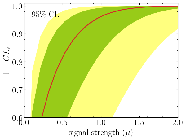
It is also possible to compute $CL_s$ value with respect to the parameter of interest, $\mu$.
This can be achieved by including a value for poi_test argument.
import matplotlib.pyplot as plt
import numpy as np

poi = np.linspace(0,10,20)
poiUL = np.array([stat_model.exclusion_confidence_level(poi_test=p, expected=spey.ExpectationType.aposteriori) for p in poi])
plt.plot(poi, poiUL[:,2], color="tab:red")
plt.fill_between(poi, poiUL[:,1], poiUL[:,3], alpha=0.8, color="green", lw=0)
plt.fill_between(poi, poiUL[:,0], poiUL[:,4], alpha=0.5, color="yellow", lw=0)
plt.plot([0,10], [.95,.95], color="k", ls="dashed")
plt.xlabel(r"${\rm signal\ strength}\ (\mu)$")
plt.ylabel("$CL_s$")
plt.xlim([0,10])
plt.ylim([0.6,1.01])
plt.text(0.5,0.96, r"$95\%\ {\rm CL}$")
plt.show()
Here in the first line, we extract $CL_s$ values per POI for spey.ExpectationType.aposteriori
expectation type, and we plot specific standard deviations, which provide the following plot:
The excluded value of POI can also be retrieved by spey.StatisticalModel.poi_upper_limitfunction, which is the exact point where the red-curve and black dashed line meet. The upper limit for the $\pm1\sigma$ or $\pm2\sigma$ bands can be extracted by settingexpected_pvalueto"1sigma"or"2sigma"`` respectively, e.g.
stat_model.poi_upper_limit(expected=spey.ExpectationType.aposteriori, expected_pvalue="1sigma")
# [0.5507713378348318, 0.9195052042538805, 1.4812721449679866]
At a lower level, one can extract the likelihood information for the statistical model by calling
spey.StatisticalModel.likelihood and spey.StatisticalModel.maximize_likelihood functions.
By default, these will return negative log-likelihood values, but this can be changed via return_nll=False
argument.
muhat_obs, maxllhd_obs = stat_model.maximize_likelihood(return_nll=False, )
muhat_apri, maxllhd_apri = stat_model.maximize_likelihood(return_nll=False, expected=spey.ExpectationType.apriori)

poi = np.linspace(-3,4,60)

llhd_obs = np.array([stat_model.likelihood(p, return_nll=False) for p in poi])
llhd_apri = np.array([stat_model.likelihood(p, expected=spey.ExpectationType.apriori, return_nll=False) for p in poi])
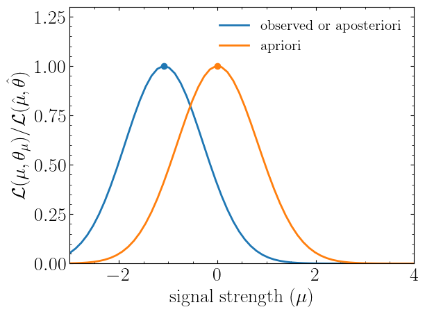
Here, in the first two lines, we extracted the maximum likelihood and the POI value that maximizes the likelihood for two different expectation types. In the following, we computed likelihood distribution for various POI values, which then can be plotted as follows
plt.plot(poi, llhd_obs/maxllhd_obs, label=r"${\rm observed\ or\ aposteriori}$")
plt.plot(poi, llhd_apri/maxllhd_apri, label=r"${\rm apriori}$")
plt.scatter(muhat_obs, 1)
plt.scatter(muhat_apri, 1)
plt.legend(loc="upper right")
plt.ylabel(r"$\mathcal{L}(\mu,\theta_\mu)/\mathcal{L}(\hat\mu,\hat\theta)$")
plt.xlabel(r"${\rm signal\ strength}\ (\mu)$")
plt.ylim([0,1.3])
plt.xlim([-3,4])
plt.show()
Notice the slight difference between likelihood distributions; this is because of the use of different expectation types.
The dots on the likelihood distribution represent the point where the likelihood is maximized. Since for a
spey.ExpectationType.apriori likelihood distribution observed and background values are the same, the likelihood
should peak at $\mu=0$.
Release history Release notifications | RSS feed


Download files
Download the file for your platform. If you're not sure which to choose, learn more about installing packages.
Source Distribution
Built Distribution
Filter files by name, interpreter, ABI, and platform.
If you're not sure about the file name format, learn more about wheel file names.
Copy a direct link to the current filters
File details
Details for the file spey-0.2.6.tar.gz.
File metadata
- Download URL: spey-0.2.6.tar.gz
- Upload date:
- Size: 89.5 kB
- Tags: Source
- Uploaded using Trusted Publishing? No
- Uploaded via: twine/6.2.0 CPython/3.9.18
File hashes
| Algorithm | Hash digest | |
|---|---|---|
| SHA256 |
8b08d53b6bf934395d04b21d3e768e86135007faf8c14acfd5af403eb90930ac
|
|
| MD5 |
60cf7a8a8ac64df6495374037428070d
|
|
| BLAKE2b-256 |
1725a2f321279c1b7e68eb12d5af6666a2a71e0367f0e4bce09172f7ccbb3da8
|
File details
Details for the file spey-0.2.6-py3-none-any.whl.
File metadata
- Download URL: spey-0.2.6-py3-none-any.whl
- Upload date:
- Size: 81.9 kB
- Tags: Python 3
- Uploaded using Trusted Publishing? No
- Uploaded via: twine/6.2.0 CPython/3.9.18
File hashes
| Algorithm | Hash digest | |
|---|---|---|
| SHA256 |
3e8b5f6cd86f5425edaee2f9ac8fe4eb6ad43e0575d5cc72d62619c286c697a9
|
|
| MD5 |
0bb9012784fad85d50667e5e8f97125d
|
|
| BLAKE2b-256 |
419600dff288d20e57d56786c1658d52719dbd8d9e3f685e58f1e58dbad8c43f
|


