sphinxcontrib-plot 1.1.11

A sphinx extension to plot graph such as ditaa, gnuplot, pyplot, etc in you sphinx document.

A sphinx extension to plot all kinds of graph such as ditaa, gnuplot, pyplot, dot, magick, blockdiag, seqdiag, actdiag, nwdiag.

The extension defines a new “.. plot::” directive.

The directive execute the given command/script and insert the generated figure into the document (like the .. image:: directive). Compared to directive “.. image::”, it generate the image at first by the given script.

For example you execute “command parameters_or_script” to generate the “command_output.png”, Writing the directive as following would include the image into you document:

.. plot command parameters_or_script
   :caption: An example

A real examples is magick as following and more examples are shown later.:

.. plot:: magick rose: -fill none -stroke white -draw 'line 5,40 65,5'  rose_raw.png
   :caption: An magick example

This is the output:

1. Installing and setup

1. Install:

   pip install sphinxcontrib-plot

2. Set “sphinx_plot_directive” to the list of extensions in the conf.py:

   extensions = ['sphinxcontrib.plot']

3. You may need to install extra command that sphinx-plot-directive depends on:

   apt install imagemagick inkscape libwebp gnuplot

2. Usage

Inlcuding a “.. plot::” code block in your sphinx document would generate the figure into the built document directly. For HTML output it’s .png(or .svg for vector), For LaTeX output, it will include a .png(or .pdf for vector), etc..

The plot content may be defined in one of Three ways:

2.1 A simple plot command to generate a figure.

.. plot:: magick rose: -fill none -stroke white -draw 'line 5,40 65,5'  rose_raw.png
   :caption: An magick example

The output is:

.

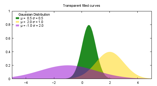
2.2 A plot command(gnuplot, ditaa, matplotlib or graphviz) with inline script

.. plot:: gnuplot
    :caption: figure 3. illustration for gnuplot

    set output "test.png"
    set terminal pngcairo size 900,600
    set style fill transparent solid 0.5 noborder
    set style function filledcurves y1=0
    Gauss(x,mu,sigma) = 1./(sigma*sqrt(2*pi)) * exp( -(x-mu)**2 / (2*sigma**2) )
    d1(x) = Gauss(x, 0.5, 0.5)
    d2(x) = Gauss(x,  2.,  1.)
    d3(x) = Gauss(x, -1.,  2.)
    set xrange [-5:5]
    set yrange [0:1]
    set key title "Gaussian Distribution"
    set key top left Left reverse samplen 1
    set title "Transparent filled curves"
    plot d1(x) fs solid 1.0 lc rgb "forest-green" title "μ =  0.5 σ = 0.5", \
         d2(x) lc rgb "gold" title "μ =  2.0 σ = 1.0", \
         d3(x) lc rgb "dark-violet" title "μ = -1.0 σ = 2.0"

The output is:

.

2.3 A plot command with included file

.. plot:: ditaa --svg
   :caption: figure 2. illustration for ditaa with option
   :include: _static/ditaa_example.txt

After compilation, the above file becomes:

2.4 inline image

for example, an icons is generated and inserted.

This is a |rose|.

.. |rose| plot:: magick rose: -fill none -stroke white -draw 'line 5,40 65,5'  rose_raw.png

The output is:

This is a .

3 Options

sphinx-plot-directive provide global options and plot image for easy use. Besides you can change the output by change the command’s own options.

3.1 global options

You can define the prefered format for different output. It’s best effort, if it couldn’t be done, the output format might be .png or anything else.:

plot_format = dict(html='svg', latex='pdf')

3.2 sphinx-plot-directive options

sphinx-plot-directive specific options:

1. caption:

   Caption of the generated figure.

2. include:

   include the plot script. Make sure it’s readable.

3. magick:

   add annotate or watermark.

4. show_source:

   for text generated iamge, if the source code is shown.

5. latex_show_max_png:

   When the build target is is latexpdf and output is .gif, We can magick it to multiple .png, then this defines how many frames would be shown in latex output. it’s integer.

Common image options:

Since plot generate figure/image, it’s in fact a image. So all the options of figure and image could be used. For example:

1. name:

   the reference name for the figure/image. For html, it would rename the output file to the @name. Since latex doesn’t do well in supporting :name: for example doesn’t support Chinese/SPACE, doesn’t generate linke to :name, we don’t do that in latex.

For example:

.. plot:: gnuplot
    :caption: figure 1. illustration for gnuplot with watermark.
    :size: 900,600
    :width: 600

    plot [-5:5] (sin(1/x) - cos(x))*erfc(x)

3.3 command options

You can add any parameter after the command. sphinxcontrib-plot doesn’t know it and only get the graph after it’s executed. for example:

.. plot:: ditaa --no-antialias -s 2
   :caption: figure 1. illustration for ditaa with option.

    +--------+   +-------+    +-------+
    |        | --+ ditaa +--> |       |
    |  Text  |   +-------+    |diagram|
    |Document|   |!magic!|    |       |
    |     {d}|   |       |    |       |
    +---+----+   +-------+    +-------+
        :                         ^
        |       Lots of work      |
        +-------------------------+

4. More Examples

In rst we we use image and figure directive to render image/figure. In fact we can plot anything in rst as it was on shell. You need only include the command or script in the directive body, then the figure would be automatically included in your sphinx document. For examples:

4.1 gnuplot example

The first example is gnuplot.:

.. plot:: gnuplot
    :caption: figure 3. illustration for gnuplot
    :image: test.png

    set output "test.png"
    set terminal pngcairo size 900,600
    set style fill transparent solid 0.5 noborder
    set style function filledcurves y1=0
    Gauss(x,mu,sigma) = 1./(sigma*sqrt(2*pi)) * exp( -(x-mu)**2 / (2*sigma**2) )
    d1(x) = Gauss(x, 0.5, 0.5)
    d2(x) = Gauss(x,  2.,  1.)
    d3(x) = Gauss(x, -1.,  2.)
    set xrange [-5:5]
    set yrange [0:1]
    set key title "Gaussian Distribution"
    set key top left Left reverse samplen 1
    set title "Transparent filled curves"
    plot d1(x) fs solid 1.0 lc rgb "forest-green" title "μ =  0.5 σ = 0.5", \
         d2(x) lc rgb "gold" title "μ =  2.0 σ = 1.0", \
         d3(x) lc rgb "dark-violet" title "μ = -1.0 σ = 2.0"

After compilation, the above file becomes:

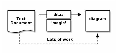
4.2 ditaa example

Another example is ditaa. ditaa is a small command-line utility that can magick diagrams drawn using ascii art into proper bitmap graphics. Ditaa is in java and we We could use following directive to render the image with extra parameters:

.. plot:: ditaa
   :caption: figure 1. illustration for ditaa

    +--------+   +-------+    +-------+
    |        | --+ ditaa +--> |       |
    |  Text  |   +-------+    |diagram|
    |Document|   |!magic!|    |       |
    |     {d}|   |       |    |       |
    +---+----+   +-------+    +-------+
        :                         ^
        |       Lots of work      |
        +-------------------------+

To render the best image, it will add –svg even user didn’t add it. The it will generate a vector image:

.. plot:: ditaa --svg
   :caption: figure 2. illustration for ditaa with option

      +--------+   +-------+    +-------+
      |        | --+ ditaa +--> |       |
      |  Text  |   +-------+    |diagram|
      |Document|   |!magic!|    |       |
      |     {d}|   |       |    |       |
      +---+----+   +-------+    +-------+
          :                         ^
          |       Lots of work      |
          +-------------------------+

After compilation, the above file becomes:

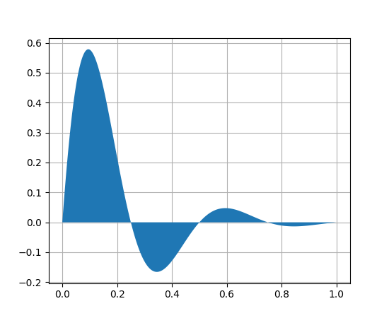
4.3 python(matplotlib) example

Another example is mulplotlib.plot.

.. plot:: python
    :caption: figure 4. illustration for python

    import numpy as np
    import matplotlib.pyplot as plt

    x = np.linspace(0, 1, 500)
    y = np.sin(4 * np.pi * x) * np.exp(-5 * x)

    fig, ax = plt.subplots()

    ax.fill(x, y, zorder=10)
    ax.grid(True, zorder=5)
    plt.show()

After compilation, we could get the following image:

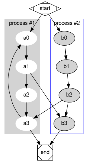
4.4 graphviz(dot) example

Another example is graphivx(dot), since we want to generate png image, we add the option in the command, it’s dot’s own option:

.. plot:: dot -Tpng
    :caption: illustration for dot

    digraph G {

            subgraph cluster_0 {
                    style=filled;
                    color=lightgrey;
                    node [style=filled,color=white];
                    a0 -> a1 -> a2 -> a3;
                    label = "process #1";
            }

            subgraph cluster_1 {
                    node [style=filled];
                    b0 -> b1 -> b2 -> b3;
                    label = "process #2";
                    color=blue
            }
            start -> a0;
            start -> b0;
            a1 -> b3;
            b2 -> a3;
            a3 -> a0;
            a3 -> end;
            b3 -> end;

            start [shape=Mdiamond];
            end [shape=Msquare];
    }

After compilation, the above file becomes:

4.5 imagemagick example

Another example is magick. You can write the command in the commnad line:

.. plot:: magick rose: -fill none -stroke white -draw 'line 5,40 65,5'  rose_raw.png
:caption: illustration for magick

This is the output:

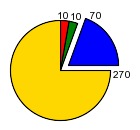
or you can write a magick script as the following:

.. plot:: magick
    :caption: illustration for magick

    magick -size 140x130 xc:white -stroke black \
        -fill red   -draw "path 'M 60,70 L   60,20   A 50,50 0 0,1 68.7,20.8 Z'" \
        -fill green -draw "path 'M 60,70 L 68.7,20.8 A 50,50 0 0,1 77.1,23.0 Z'" \
        -fill blue  -draw "path 'M 68,65 L 85.1,18.0 A 50,50 0 0,1  118,65   Z'" \
        -fill gold  -draw "path 'M 60,70 L  110,70   A 50,50 0 1,1   60,20   Z'" \
        -fill black -stroke none  -pointsize 10 \
        -draw "text 57,19 '10' text 70,20 '10' text 90,19 '70' text 113,78 '270'" \
        out.png

This is the output:

4.6 blockdiag, seqdiag, actdiag, nwdiag.

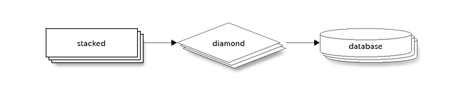
demo for blockdiag:

.. plot:: blockdiag
    :caption: demo for blockdiag
    :name: demo for blockdiag

    blockdiag {
      // Set stacked to nodes.
      stacked [stacked];
      diamond [shape = "diamond", stacked];
      database [shape = "flowchart.database", stacked];

      stacked -> diamond -> database;
    }

This will generate the follong image on your .htm/.pdf document generated from sphinx:

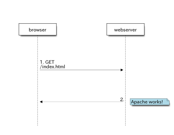
demo for seqdiag:

.. plot:: blockdiag
    :caption: demo for seqdiag
    :name: demo for seqdiag

    seqdiag {
      // Set edge metrix.
      edge_length = 300;  // default value is 192
      span_height = 80;  // default value is 40

      // Set fontsize.
      default_fontsize = 16;  // default value is 11

      // Do not show activity line
      activation = none;

      // Numbering edges automaticaly
      autonumber = True;

      // Change note color
      default_note_color = lightblue;

      browser  -> webserver [label = "GET \n/index.html"];
      browser <-- webserver [note = "Apache works!"];
    }

This will generate the follong image on your .htm/.pdf document generated from sphinx:

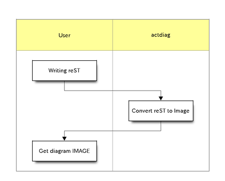
demo for actdiag:

.. plot:: actdiag
    :caption: demo for actdiag

    actdiag {
      write -> convert -> image

      lane user {
         label = "User"
         write [label = "Writing reST"];
         image [label = "Get diagram IMAGE"];
      }
      lane actdiag {
         convert [label = "convert reST to Image"];
      }
    }

This will generate the follong image on your .htm/.pdf document generated from sphinx:

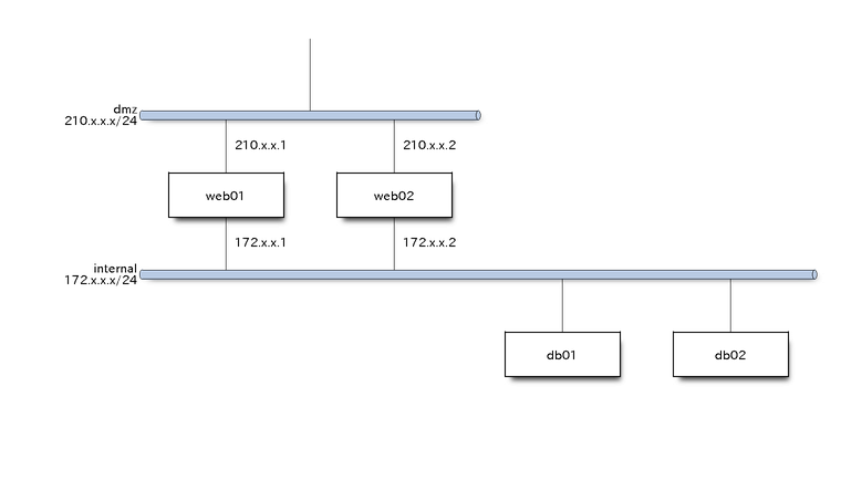
demo for nwdiag:

.. plot:: nwdiag
    :caption: demo for actdiag

    nwdiag {
      network dmz {
          address = "210.x.x.x/24"

          web01 [address = "210.x.x.1"];
          web02 [address = "210.x.x.2"];
      }
      network internal {
          address = "172.x.x.x/24";

          web01 [address = "172.x.x.1"];
          web02 [address = "172.x.x.2"];
          db01;
          db02;
      }
    }

This will generate the follong image on your .htm/.pdf document generated from sphinx:

4.7 svg

We can include the .svg image in our document directly and it will be rended as a picture in either html or pdf output.:

.. plot:: svg

    <svg version="1.1"
         baseProfile="full"
         width="300" height="200"
         xmlns="http://www.w3.org/2000/svg">
      <rect width="100%" height="100%" fill="red" />
      <circle cx="150" cy="100" r="80" fill="green" />
      <text x="150" y="125" font-size="60" text-anchor="middle" fill="white">SVG</text>
    </svg>

You can use “:include:” parameter to include a .svg image:

.. plot:: svg
    :include: _static/test.svg
    :caption: include参数的用法

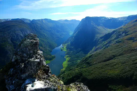
4.8 use cp to include .webp into the document

We can copy the .dwep picture into the document directly, it would be rended as .webp in html and .png in latexpdf.:

.. plot:: cp _static/palms.webp out.webp
    :caption: An example to include .webp picture.

4.9 use wget/curl to include web image

We can include webp image into the document directly. It would download it at the first time and copy it to _static/ automaticallly the first time. Next time it would use the cache.:

.. plot:: wget https://www.gstatic.com/webp/gallery/1.webp
    :caption: An example to wget

This will generate the .webp image on your .html document and it will be converted .png in pdf output automatically:

The above directive do the follwing thing at the first time:

wget https://www.gstatic.com/webp/gallery/1.webp
cp 1.webp _static/

And do the following thing the next time:

cp _static/1.webp .

5. License

MIT

6. Changelog

1.0 Initial upload.

1.0.8 Bug fix: When there is no :size: in gnuplot plot, it might crash.

1.0.10 Bug fix: fix the issue that magick doesn’t work.

1.0.13 Support magick script

1.0.17 bug fix: magick can has no body.

1.0.18 New feature: 1) Support montage command; 2) Support including .gif image into html and pdf. If it’s html, play the .gif, or else if it’s pdf, magick the .gif to a list of frame.

1.0.19 Support lines starting with # in the magick/montage body.

1.1.0 Bug fix: It doesn’t work for ditaa with magick parameters.

1.1.1 Support the following plot command: blockdiag, seqdiag, actdiag, nwdiag.

1.1.2 magick command must be in command line or in content with one worad “magick” in command line.

1.1.3 Bug fix: make html might cause the following error: AttributeError: ‘str’ object has no attribute ‘extend’

1.1.4 Support inline image.

1.1.5 When the output is .gif, print the frames in 8 frames in every row by default.

1.1.6 When .gif is given width, then increase it in latexpdf output.

1.1.7 Support new commands: dwebp and others.

1.1.8 Support new command cp to incluce .webp.

1.1.9 Support new command wget/curl.

1.1.10 Bug fix: Sometimes it crash when there is other sphinxcontrib plugin in the same documents.

1.1.11 Bug fix: When command is in a relative path, it couldn’t work.

Refenreces

1. gnuplot, http://www.gnuplot.info/

2. ditaa, https://github.com/tmthrgd/ditaa-ditaa

3. Matplotlib, https://matplotlib.org/

4. graphviz, https://graphviz.org/

5. imagemagick, https://imagemagick.org

6. blockdiag, http://blockdiag.com/en/blockdiag/index.html

7. seqdiag , http://blockdiag.com/en/seqdiag/index.html

8. actdiag , http://blockdiag.com/en/nwdiag/actdiag.html

9. nwdiag , http://blockdiag.com/en/nwdiag/index.html