Awesome Spectral Indices in Python
Verified details
These details have been verified by PyPIProject links
GitHub Statistics
Maintainers

Project description

Awesome Spectral Indices in Python:
Numpy | Pandas | GeoPandas | Xarray | Earth Engine | Planetary Computer | Dask | Cupy | Cupy-Xarray


GitHub: https://github.com/davemlz/spyndex
Documentation: https://spyndex.readthedocs.io/
Paper: https://doi.org/10.1038/s41597-023-02096-0
PyPI: https://pypi.org/project/spyndex/
Conda-forge: https://anaconda.org/conda-forge/spyndex
Tutorials: https://spyndex.readthedocs.io/en/latest/tutorials.html
Citation
If you use this work, please consider citing the following paper:
@article{montero2023standardized,
  title={A standardized catalogue of spectral indices to advance the use of remote sensing in Earth system research},
  author={Montero, David and Aybar, C{\'e}sar and Mahecha, Miguel D and Martinuzzi, Francesco and S{\"o}chting, Maximilian and Wieneke, Sebastian},
  journal={Scientific Data},
  volume={10},
  number={1},
  pages={197},
  year={2023},
  publisher={Nature Publishing Group UK London}
}
Overview
The Awesome Spectral Indices is a standardized ready-to-use curated list of spectral indices that can be used as expressions for computing spectral indices in remote sensing applications. The list was born initially to supply spectral indices for Google Earth Engine through eemont and spectral, but given the necessity to compute spectral indices for other object classes outside the Earth Engine ecosystem, a new package was required.
Spyndex is a python package that uses the spectral indices from the Awesome Spectral Indices list and creates an expression evaluation method that is compatible with python object classes that support overloaded operators (e.g. numpy.ndarray, pandas.Series, xarray.DataArray).
Some of the spyndex features are listed here:
- Access to Spectral Indices from the Awesome Spectral Indices list.
- Multiple Spectral Indices computation.
- Kernel Indices computation.
- Parallel processing.
- Compatibility with a lot of python objects!
Check the simple usage of spyndex here:
import spyndex
import numpy as np
import xarray as xr

N = np.random.normal(0.6,0.10,10000)
R = np.random.normal(0.1,0.05,10000)

da = xr.DataArray(
    np.array([N,R]).reshape(2,100,100),
    dims = ("band","x","y"),
    coords = {"band": ["NIR","Red"]}
)

idx = spyndex.computeIndex(
    index = ["NDVI","SAVI"],
    params = {
        "N": da.sel(band = "NIR"),
        "R": da.sel(band = "Red"),
        "L": 0.5
    }
)
Bands can also be passed as keywords arguments:
idx = spyndex.computeIndex(
    index = ["NDVI","SAVI"],
    N = da.sel(band = "NIR"),
    R = da.sel(band = "Red"),
    L = 0.5
)
And indices can be computed from their class:
idx = spyndex.indices.NDVI.compute(
    N = da.sel(band = "NIR"),
    R = da.sel(band = "Red"),
)
How does it work?
Any python object class that supports overloaded operators can be used with spyndex methods.
"Hey... what do you mean by 'overloaded operators'?"
That's the million dollars' question! An object class that supports overloaded operators is the one that allows you to compute mathematical
operations using common operators (+, -, /, *, **) like a + b, a + b * c or (a - b) / (a + b). You know the last one, right? That's
the formula of the famous NDVI.
So, if you can use the overloaded operators with an object class, you can use that class with spyndex!
BE CAREFUL! Not all overloaded operators work as mathematical operators. In a
listobject class, the addition operator (+) concatenates two objects instead of performing an addition operation! So you must convert thelistinto anumpy.ndarraybefore using spyndex!
Here is a little list of object classes that support mathematical overloaded operators:
float(Python Built-in type) ornumpy.float*(with numpy)int(Python Built-in type) ornumpy.int*(with numpy)numpy.ndarray(with numpy)pandas.Series(with pandas or geopandas)xarray.DataArray(with xarray)ee.Image(with earthengine-api and eemont)ee.Number(with earthengine-api and eemont)
And wait, there is more! If objects that support overloaded operatores can be used in spyndex, that means that you can work in parallel with dask!
Here is the list of the dask objects that you can use with spyndex:
BUT WAIT! THERE IS EVEN MORE! If you want GPU-accelerated computing, you can use cupy!
cupy.ndarray(with cupy or with cupy-xarray)
This means that you can actually use spyndex in a lot of processes! For example, you can download a Sentinel-2 image with
sentinelsat, open and read it with rasterio and then compute
the desired spectral indices with spyndex. Or you can search through the Landsat-8 STAC in the
Planetary Computer ecosystem using pystac-client,
convert it to an xarray.DataArray with stackstac and then compute spectral indices using
spyndex in parallel with dask or with GPU acceleration using cupy! Amazing, right!?
Installation
Install the latest version from PyPI:
pip install spyndex
Upgrade spyndex by running:
pip install -U spyndex
Install the latest version from conda-forge:
conda install -c conda-forge spyndex
Install the latest dev version from GitHub by running:
pip install git+https://github.com/davemlz/spyndex
Features
Exploring Spectral Indices
Spectral Indices from the Awesome Spectral Indices list can be accessed through
spyndex.indices. This is a Box object where each one of the indices in the list
can be accessed as well as their attributes:
import spyndex

# All indices
spyndex.indices

# NDVI index
spyndex.indices["NDVI"]

# Or with dot notation
spyndex.indices.NDVI

# Formula of the NDVI
spyndex.indices["NDVI"]["formula"]

# Or with dot notation
spyndex.indices.NDVI.formula

# Reference of the NDVI
spyndex.indices["NDVI"]["reference"]

# Or with dot notation
spyndex.indices.NDVI.reference
Default Values
Some Spectral Indices require constant values in order to be computed. Default values
can be accessed through spyndex.constants. This is a Box object where each one
of the constants can be
accessed:
import spyndex

# All constants
spyndex.constants

# Canopy Background Adjustment
spyndex.constants["L"]

# Or with dot notation
spyndex.constants.L

# Default value
spyndex.constants["L"]["default"]

# Or with dot notation
spyndex.constants.L.default
Band Parameters
The standard band parameters description can be accessed through spyndex.bands. This is
a Box object where each one of the bands
can be accessed:
import spyndex

# All bands
spyndex.bands

# Blue band
spyndex.bands["B"]

# Or with dot notation
spyndex.bands.B
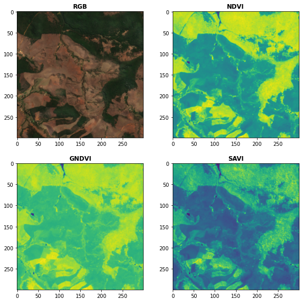
One (or more) Spectral Indices Computation
Use the computeIndex() method to compute as many spectral indices as you want!
The index parameter receives the spectral index or a list of spectral indices to
compute, while the params parameter receives a dictionary with the
required parameters
for the spectral indices computation.
import spyndex
import xarray as xr
import matplotlib.pyplot as plt
from rasterio import plot

# Open a dataset (in this case a xarray.DataArray)
snt = spyndex.datasets.open("sentinel")

# Scale the data (remember that the valid domain for reflectance is [0,1])
snt = snt / 10000

# Compute the desired spectral indices
idx = spyndex.computeIndex(
    index = ["NDVI","GNDVI","SAVI"],
    params = {
        "N": snt.sel(band = "B08"),
        "R": snt.sel(band = "B04"),
        "G": snt.sel(band = "B03"),
        "L": 0.5
    }
)

# Plot the indices (and the RGB image for comparison)
fig, ax = plt.subplots(2,2,figsize = (10,10))
plot.show(snt.sel(band = ["B04","B03","B02"]).data / 0.3,ax = ax[0,0],title = "RGB")
plot.show(idx.sel(index = "NDVI").data,ax = ax[0,1],title = "NDVI")
plot.show(idx.sel(index = "GNDVI").data,ax = ax[1,0],title = "GNDVI")
plot.show(idx.sel(index = "SAVI").data,ax = ax[1,1],title = "SAVI")
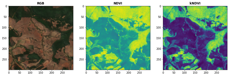
Kernel Indices Computation
Use the computeKernel() method to compute the required kernel for kernel indices like
the kNDVI! The kernel parameter receives the kernel to compute, while the params
parameter receives a dictionary with the
required parameters
for the kernel computation (e.g., a, b and sigma for the RBF kernel).
import spyndex
import xarray as xr
import matplotlib.pyplot as plt
from rasterio import plot

# Open a dataset (in this case a xarray.DataArray)
snt = spyndex.datasets.open("sentinel")

# Scale the data (remember that the valid domain for reflectance is [0,1])
snt = snt / 10000

# Compute the kNDVI and the NDVI for comparison
idx = spyndex.computeIndex(
    index = ["NDVI","kNDVI"],
    params = {
        # Parameters required for NDVI
        "N": snt.sel(band = "B08"),
        "R": snt.sel(band = "B04"),
        # Parameters required for kNDVI
        "kNN" : 1.0,
        "kNR" : spyndex.computeKernel(
            kernel = "RBF",
            params = {
                "a": snt.sel(band = "B08"),
                "b": snt.sel(band = "B04"),
                "sigma": snt.sel(band = ["B08","B04"]).mean("band")
            }),
    }
)

# Plot the indices (and the RGB image for comparison)
fig, ax = plt.subplots(1,3,figsize = (15,15))
plot.show(snt.sel(band = ["B04","B03","B02"]).data / 0.3,ax = ax[0],title = "RGB")
plot.show(idx.sel(index = "NDVI").data,ax = ax[1],title = "NDVI")
plot.show(idx.sel(index = "kNDVI").data,ax = ax[2],title = "kNDVI")
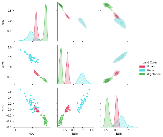
A pandas.DataFrame? Sure!
No matter what kind of python object you're working with, it can be used with spyndex as long as it supports mathematical overloaded operators!
import spyndex
import pandas as pd
import seaborn as sns
import matplotlib.pyplot as plt

# Open a dataset (in this case a pandas.DataFrame)
df = spyndex.datasets.open("spectral")

# Compute the desired spectral indices
idx = spyndex.computeIndex(
    index = ["NDVI","NDWI","NDBI"],
    params = {
        "N": df["SR_B5"],
        "R": df["SR_B4"],
        "G": df["SR_B3"],
        "S1": df["SR_B6"]
    }
)

# Add the land cover column to the result
idx["Land Cover"] = df["class"]

# Create a color palette for plotting
colors = ["#E33F62","#3FDDE3","#4CBA4B"]

# Plot a pairplot to check the indices behaviour
plt.figure(figsize = (15,15))
g = sns.PairGrid(idx,hue = "Land Cover",palette = sns.color_palette(colors))
g.map_lower(sns.scatterplot)
g.map_upper(sns.kdeplot,fill = True,alpha = .5)
g.map_diag(sns.kdeplot,fill = True)
g.add_legend()
plt.show()
Parallel Processing
Parallel processing is possible with spyndex and dask! You can use dask.array or dask.dataframe objects to compute spectral indices with spyndex!
If you're using xarray, you can also define a chunk size and work in parallel!
import spyndex
import numpy as np
import dask.array as da

# Define the array shape
array_shape = (10000,10000)

# Define the chunk size
chunk_size = (1000,1000)

# Create a dask.array object
dask_array = da.array([
    da.random.normal(0.6,0.10,array_shape,chunks = chunk_size),
    da.random.normal(0.1,0.05,array_shape,chunks = chunk_size)
])

# "Compute" the desired spectral indices
idx = spyndex.computeIndex(
    index = ["NDVI","SAVI"],
    params = {
        "N": dask_array[0],
        "R": dask_array[1],
        "L": 0.5
    }
)

# Since dask works in lazy mode,
# you have to tell it that you want to compute the indices!
idx.compute()
Using cupy
You want GPU-accelerated computing? Well, that's also possible with spyndex and cupy (and with cupy-xarray too!).
Try it with cupy:
import spyndex
import cupy as cp

# cupy.ndarray objects
N = cp.random.normal(0.6,0.10,10000)
R = cp.random.normal(0.1,0.05,10000)

# Returns a cupy.ndarray object
idx = spyndex.computeIndex(
    index = "NDVI",
    N = N,
    R = R
)
Try it with cupy-xarray:
import spyndex
import xarray as xr
import cupy_xarray

# Open a dataset (in this case a xarray.DataArray)
snt = spyndex.datasets.open("sentinel")

# Convert it to a dataset of cupy.ndarray objects
snt_cupy = snt.cupy.as_cupy()

# Scale the data (remember that the valid domain for reflectance is [0,1])
snt_cupy = snt_cupy / 10000

# Compute the desired spectral indices
idx_cupy = spyndex.computeIndex(
    index = ["NDVI","GNDVI","SAVI"],
    params = {
        "N": snt_cupy.sel(band = "B08"),
        "R": snt_cupy.sel(band = "B04"),
        "G": snt_cupy.sel(band = "B03"),
        "L": 0.5
    }
)

# Convert back to numpy!
idx = idx_cupy.as_numpy()
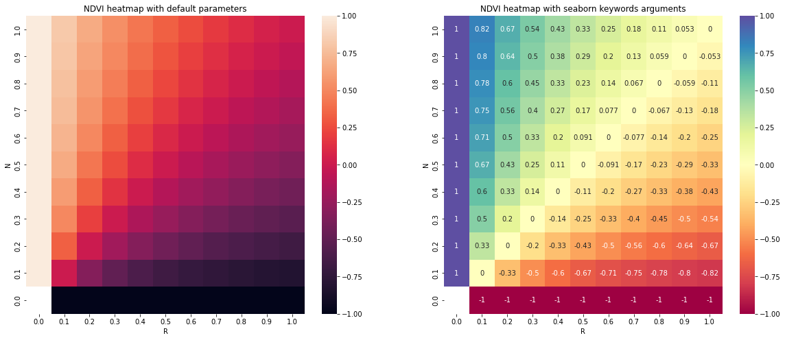
Plotting Spectral Indices
All posible values of a spectral index can be visualized using spyndex.plot.heatmap()! This is a module that doesn't require data,
just specify the index, the bands, and BOOM! Heatmap of all the possible values of the index!
import spyndex
import matplotlib.pyplot as plt
import seaborn as sns

# Define subplots grid
fig, ax = plt.subplots(1,2,figsize = (20,8))

# Plot the NDVI with the Red values on the x-axis and the NIR on the y-axis
ax[0].set_title("NDVI heatmap with default parameters")
spyndex.plot.heatmap("NDVI","R","N",ax = ax[0])

# Keywords arguments can be passed for sns.heatmap()
ax[1].set_title("NDVI heatmap with seaborn keywords arguments")
spyndex.plot.heatmap("NDVI","R","N",annot = True,cmap = "Spectral",ax = ax[1])

plt.show()
License
The project is licensed under the MIT license.
Contributing
Check the contributing page.
Project details
Verified details
These details have been verified by PyPIProject links
GitHub Statistics
Maintainers
Release history Release notifications | RSS feed


Download files
Download the file for your platform. If you're not sure which to choose, learn more about installing packages.
Source Distribution
Built Distribution
Filter files by name, interpreter, ABI, and platform.
If you're not sure about the file name format, learn more about wheel file names.
Copy a direct link to the current filters
File details
Details for the file spyndex-0.10.0.tar.gz.
File metadata
- Download URL: spyndex-0.10.0.tar.gz
- Upload date:
- Size: 732.9 kB
- Tags: Source
- Uploaded using Trusted Publishing? Yes
- Uploaded via: twine/6.1.0 CPython/3.13.7
File hashes
| Algorithm | Hash digest | |
|---|---|---|
| SHA256 |
039c3b9bd0b24613e03aa26b79a44aee677d6722c68c5dbed6686a833432e3e0
|
|
| MD5 |
28891a9cc4650f9df7d29bd5978e17a7
|
|
| BLAKE2b-256 |
6b3eaa3eb9720b8e38c7cef23c3d581a2689090af2758cc79b544bc3e41df5e0
|
Provenance
The following attestation bundles were made for spyndex-0.10.0.tar.gz:
Publisher:
publish.yml on awesome-spectral-indices/spyndex
-
Statement:
-
Statement type:
https://in-toto.io/Statement/v1 -
Predicate type:
https://docs.pypi.org/attestations/publish/v1 -
Subject name:
spyndex-0.10.0.tar.gz -
Subject digest:
039c3b9bd0b24613e03aa26b79a44aee677d6722c68c5dbed6686a833432e3e0 - Sigstore transparency entry: 1203854478
- Sigstore integration time:
-
Permalink:
awesome-spectral-indices/spyndex@5bafeea1e78c7577664ff4d7ede53b0fb1823c5e -
Branch / Tag:
refs/tags/0.10.0 - Owner: https://github.com/awesome-spectral-indices
-
Access:
public
-
Token Issuer:
https://token.actions.githubusercontent.com -
Runner Environment:
github-hosted -
Publication workflow:
publish.yml@5bafeea1e78c7577664ff4d7ede53b0fb1823c5e -
Trigger Event:
release
-
Statement type:
File details
Details for the file spyndex-0.10.0-py3-none-any.whl.
File metadata
- Download URL: spyndex-0.10.0-py3-none-any.whl
- Upload date:
- Size: 771.4 kB
- Tags: Python 3
- Uploaded using Trusted Publishing? Yes
- Uploaded via: twine/6.1.0 CPython/3.13.7
File hashes
| Algorithm | Hash digest | |
|---|---|---|
| SHA256 |
127118c93fb265964273d35656c3413bd5cfdc00861b188b8f12c3c7a58ce4d5
|
|
| MD5 |
dd48109d220eb1ce577c6fc9b43ccac0
|
|
| BLAKE2b-256 |
da2eff017d3cb5e7fe71287a8012cd8f8404a8baa9c32a1b79ae9546ac207ed3
|
Provenance
The following attestation bundles were made for spyndex-0.10.0-py3-none-any.whl:
Publisher:
publish.yml on awesome-spectral-indices/spyndex
-
Statement:
-
Statement type:
https://in-toto.io/Statement/v1 -
Predicate type:
https://docs.pypi.org/attestations/publish/v1 -
Subject name:
spyndex-0.10.0-py3-none-any.whl -
Subject digest:
127118c93fb265964273d35656c3413bd5cfdc00861b188b8f12c3c7a58ce4d5 - Sigstore transparency entry: 1203854484
- Sigstore integration time:
-
Permalink:
awesome-spectral-indices/spyndex@5bafeea1e78c7577664ff4d7ede53b0fb1823c5e -
Branch / Tag:
refs/tags/0.10.0 - Owner: https://github.com/awesome-spectral-indices
-
Access:
public
-
Token Issuer:
https://token.actions.githubusercontent.com -
Runner Environment:
github-hosted -
Publication workflow:
publish.yml@5bafeea1e78c7577664ff4d7ede53b0fb1823c5e -
Trigger Event:
release
-
Statement type:


