
stable-cart




Fit a model twice on two samples from the same population and you get two
different models. stable-cart tells you how much that would have changed the
prediction for any particular case. It refits your whole model-building
procedure on bootstrap resamples of the training data, predicts the same
evaluation cases every time, and reports the spread case by case.
The case-by-case part is the point. A logistic pipeline on scikit-learn's wine data disagrees with its own full-data fit on 1.1% of predictions on average. The 90th percentile of that disagreement is zero, and for the worst single case it is 28%: almost all the instability sits in a handful of people, and the average hides them.
The package measures instability; it does not remove it.
RepresentativeEstimator is the closest thing here to an intervention, and the
evidence for it is task-specific and reported below.
Install
pip install stable-cart
Plots need matplotlib, which is an optional extra:
pip install "stable-cart[plots]"
Audit a procedure
from sklearn.datasets import load_diabetes
from sklearn.linear_model import Ridge
from sklearn.model_selection import train_test_split
from sklearn.pipeline import make_pipeline
from sklearn.preprocessing import StandardScaler

from stable_cart import bootstrap_instability

X, y = load_diabetes(return_X_y=True)
X_train, X_eval, y_train, _ = train_test_split(X, y, test_size=0.3, random_state=0)

result = bootstrap_instability(
    lambda: make_pipeline(StandardScaler(), Ridge(alpha=1.0)),
    X_train,
    y_train,
    X_eval,
    task="continuous",
    n_bootstrap=500,
    random_state=0,
)
instability_mean             93.74
instability_p90              146.2
instability_max              433.2
mape                         7.461
mape_standard_error          0.08255
pairwise_mean                187.5
pairwise_standard_error      4.14
n_fit_attempts               501
n_resample_attempts          500
n_rejected_resamples         0
The diabetes target runs from 25 to 346. A refit's prediction for one of the 133 evaluation patients differs from the shipped model's by 7.5 units on average, and the variance of a patient's prediction across refits averages 94, about ten units of standard deviation. For the least stable patient that variance is 433, a standard deviation of 21, so a shipped prediction of 150 sits inside a two-standard-deviation band running from 108 to 192.
The two comparison numbers answer different questions. mape compares each
refit with the model you actually shipped, and pairwise_mean compares two
refits with each other. The instability_* keys summarize a per-case
statistic, and the spread across those three is usually the story: read the
maximum, not just the mean. The standard errors are Monte Carlo error from
using finitely many resamples, not sampling uncertainty over training sets, so
they tell you when to raise n_bootstrap and nothing else.
What goes inside the factory is what gets measured. Everything in the callable
is repeated on every resample; everything outside it is frozen. Standardizing
or tuning hyperparameters outside the factory measures how estimation varies
given a preprocessing choice that was itself data-dependent, which is a much
narrower question than most people mean to ask. random_state seeds the
resampling only, so seed the estimator inside the factory when you want
sampling variation isolated.
bootstrap_predictions returns the same audit without the summarizing, so a
different summary costs no further fitting.
Classification
Class labels are names. They have no spacing, so the variance of their integer codes means nothing, and neither does the variance of the winning probability. The package measures label disagreement or movement in the full probability vector, and never anything else.
from sklearn.datasets import load_wine
from sklearn.linear_model import LogisticRegression
from sklearn.model_selection import train_test_split
from sklearn.pipeline import make_pipeline
from sklearn.preprocessing import StandardScaler

from stable_cart import bootstrap_instability

X, y = load_wine(return_X_y=True)
X_train, X_eval, y_train, _ = train_test_split(
    X, y, test_size=0.3, random_state=0, stratify=y
)


def procedure():
    return make_pipeline(StandardScaler(), LogisticRegression(max_iter=2000))


labels = bootstrap_instability(
    procedure,
    X_train,
    y_train,
    X_eval,
    task="categorical",
    n_bootstrap=500,
    random_state=0,
)

probabilities = bootstrap_instability(
    procedure,
    X_train,
    y_train,
    X_eval,
    task="categorical",
    prediction_method="predict_proba",
    n_bootstrap=500,
    random_state=0,
)
                          labels   probabilities
instability_mean         0.01126        0.005527
instability_p90                0         0.01027
instability_max            0.284          0.1122
pairwise_mean            0.01763         0.01105
The label audit says two independent refits assign different classes to the same bottle of wine 1.8% of the time. The probability audit says the same bottle's probability vector moves by 0.011 in squared Euclidean distance. The label view is what a downstream decision sees. The probability view also catches movement that never crosses a decision boundary, which makes it the more sensitive instrument and the harder one to act on.
Probability columns are aligned through each refitted estimator's classes_,
including when a resample happens to omit a class, so results do not change if
you rename or renumber the classes.
Resampling is the ordinary pairs bootstrap, so class prevalence varies across
draws, as it should: freezing it understates instability. The one exception is
a draw containing a single class, which most classifiers are undefined on.
Those draws are redrawn under one estimator-independent policy, so every
configuration in a comparison faces the same conditional bootstrap
distribution, and the count of rejections comes back in
n_rejected_resamples.
Correlated rows
Patients within hospitals, repeated measures per subject, students within
classrooms: when rows are correlated, resampling them independently breaks the
correlation and the audit reports a model far steadier than it is. Pass
groups= and clusters are resampled instead, each drawn cluster taken whole.
import numpy as np
from sklearn.linear_model import LinearRegression

from stable_cart import bootstrap_instability

rng = np.random.default_rng(0)
n_hospitals, per_hospital = 40, 25
hospital = np.repeat(np.arange(n_hospitals), per_hospital)
X_train = rng.normal(size=(n_hospitals * per_hospital, 4))
y_train = (
    X_train @ np.arange(1.0, 5.0)
    + np.repeat(
        rng.normal(scale=3.0, size=n_hospitals), per_hospital
    )  # hospital effect
    + rng.normal(size=n_hospitals * per_hospital)
)
X_eval = rng.normal(size=(60, 4))

audit = bootstrap_instability(
    LinearRegression,
    X_train,
    y_train,
    X_eval,
    task="continuous",
    n_bootstrap=300,
    random_state=0,
    groups=hospital,
)
Here the hospital effect is three times the idiosyncratic noise. Generating 25 such datasets and comparing both schemes with the variance of predictions across independently generated datasets, which is the quantity the audit estimates:
truth (independent datasets)     0.2641
row bootstrap                    0.0495    0.19x   range 0.12x to 0.30x
cluster bootstrap                0.2609    0.99x   range 0.54x to 1.69x
The row bootstrap is not slightly off. It reports a fifth of the real figure,
and no dataset in the 25 got it above 0.30x. Dropping groups= is not a
conservative simplification, it is a wrong answer.
The cluster bootstrap removes that bias without manufacturing information, and the range is the honest half of the result: the single run in the code block above returns 0.343, not 0.261. Forty clusters is forty observations as far as this estimate is concerned. Read the Monte Carlo standard error, and treat a study with few clusters as the small sample it is.
stability_frontier takes groups= too, and switches its internal split to a
grouped one so no cluster lands on both sides of it.
Compare configurations on both axes
stability_frontier sweeps a parameter grid and returns the configurations
that no other configuration beats on both validation score and instability.
The same resampled index sets are reused for every configuration, so the
comparison is paired.
from sklearn.datasets import load_diabetes
from sklearn.linear_model import Ridge
from sklearn.model_selection import train_test_split
from sklearn.pipeline import make_pipeline
from sklearn.preprocessing import StandardScaler

from stable_cart import stability_frontier

X, y = load_diabetes(return_X_y=True)
X_train, X_validation, y_train, y_validation = train_test_split(
    X, y, test_size=0.3, random_state=0
)

frontier = stability_frontier(
    lambda **params: make_pipeline(StandardScaler(), Ridge(**params)),
    {"alpha": [0.01, 0.1, 1.0, 10.0, 100.0, 1000.0]},
    X_train,
    y_train,
    X_eval=X_validation,
    y_eval=y_validation,
    task="continuous",
    n_bootstrap=200,
    random_state=0,
)
alpha        r2    pairwise    on frontier
 0.01     0.393       196.2
 0.1      0.393       194.5
 1.0      0.392       183.5
10.0      0.392       155.3
100.0     0.407        92.6        yes
1000.0    0.292        38.0        yes
Ridge at alpha=100 is free money: it is the most accurate configuration on
the grid and 40% less unstable than alpha=10. alpha=1000 is a real trade,
giving up 0.115 of R-squared to cut instability by another factor of 2.4.
Everything below alpha=100 is dominated, which is the useful output of the
sweep: those four configurations are worse on both axes and there is no reason
to argue about them.
Two warnings come with this. The reported score is a validation score used to build the frontier, so it is optimistic as a performance estimate; measure the configuration you pick on untouched data or in an outer resampling loop. And a model that ignores its training data has an instability of exactly zero, so the frontier is only meaningful read across both axes at once.
See where the movement is
import matplotlib.pyplot as plt
from sklearn.datasets import load_diabetes
from sklearn.model_selection import train_test_split
from sklearn.tree import DecisionTreeRegressor

from stable_cart import (
    bootstrap_predictions,
    plot_mape_by_prediction,
    plot_prediction_instability,
)

X, y = load_diabetes(return_X_y=True)
X_train, X_eval, y_train, _ = train_test_split(X, y, test_size=0.3, random_state=0)

raw = bootstrap_predictions(
    lambda: DecisionTreeRegressor(max_depth=3, random_state=0),
    X_train,
    y_train,
    X_eval,
    task="continuous",
    n_bootstrap=200,
    random_state=0,
)

fig, axes = plt.subplots(1, 2, figsize=(11, 4.2))
plot_prediction_instability(raw, ax=axes[0])
plot_mape_by_prediction(raw, ax=axes[1])
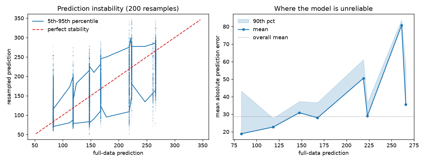
One dot is one patient under one resample. The left panel puts the full-data prediction on the horizontal axis and the resampled prediction on the vertical one, so a perfectly stable procedure would draw the diagonal. A tree predicts one value per leaf, which is why the cloud is made of vertical stripes, and the stripes are tall: a patient the full-data tree scores at 220 gets scores between 110 and 280 from the middle 90% of the resampled trees. The right panel bins the same information against the predicted value and shows that the movement is concentrated at the top of the range, where the decisions usually are.
plot_stability_frontier draws the score-instability plane for one or more
model families, with each family's Pareto set joined by a line and the
configurations it dominates left hollow.
Does the explanation hold still?
A single tree is usually chosen because someone will read it. Prediction stability says nothing about whether the reading survives a resample, and the two can move in opposite directions: when two features carry the same information, the tree flips between them on every resample while its predictions barely change.
from sklearn.tree import DecisionTreeRegressor
from sklearn.utils import resample

from stable_cart import explanation_instability, path_agreement, root_agreement

trees = [
    DecisionTreeRegressor(max_depth=3, random_state=0).fit(
        *resample(X_train, y_train, replace=True, random_state=seed)
    )
    for seed in range(200)
]

root_agreement(trees)  # 0.500
path_agreement(trees, X_eval)  # 0.124
explanation_instability(trees, max_depth=2)  # jaccard_mean 0.541
Half the resampled trees open on a different feature than the modal one, and only 12% of patients are routed through the same sequence of questions as the modal path for that patient. The predictions of these trees are moderately unstable; the explanation is worthless. That gap is the reason the two are measured separately.
Pick one model out of a resampled pool
RepresentativeEstimator fits a pool of candidates on bootstrap samples and
keeps the one closest to the pool's mean prediction on a held-out selection
split. With squared distance, that is the prediction medoid: the candidate with
the smallest average squared distance to every other candidate. The rule is
prior art, not a new algorithm.
from sklearn.datasets import load_wine
from sklearn.linear_model import LogisticRegression
from sklearn.model_selection import train_test_split
from sklearn.pipeline import make_pipeline
from sklearn.preprocessing import StandardScaler

from stable_cart import RepresentativeEstimator

X, y = load_wine(return_X_y=True)
X_train, X_test, y_train, y_test = train_test_split(
    X, y, test_size=0.3, random_state=0, stratify=y
)

representative = RepresentativeEstimator(
    estimator=make_pipeline(StandardScaler(), LogisticRegression(max_iter=2000)),
    task="classification",
    n_candidates=20,
    random_state=0,
).fit(X_train, y_train)

representative.predict(X_test)
representative.selected_index_  # 2
representative.proximity_metric_  # 'probability_mse'
It clones any scikit-learn-compatible estimator, handles multiclass, passes scikit-learn's maintained estimator checks in both regression and classification modes, and is not tree-specific.
Whether picking the medoid instead of the best-scoring candidate is worth doing depends on the task, and the evidence is uneven. A study run against a frozen pre-analysis plan compared medoid selection with best-validation selection from the same pool of 12 candidates, over 288 synthetic datasets in 12 design cells. Instability fell in all 12 cells, by 9.2% on average (95% interval -10.2% to -8.1%), but the cells differ:
| Base estimator and task | Instability | Score difference |
|---|---|---|
| Linear classification | -17.5% | +0.03 accuracy points |
| Tree classification | -12.7% | -1.08 accuracy points |
| Tree regression | -4.7% | +0.004 R-squared |
| Linear regression | -1.7% | 0.000 R-squared |
Linear classification is the clear case. Tree regression gains a little at no
cost. Tree classification pays about a point of accuracy, which broke the
guardrail the study fixed in advance. For linear regression the instability
interval spans zero, so there is nothing to claim. Treat this as task-specific
evidence, not a general result, and audit your own case with
bootstrap_instability.
Check the resampler against a known answer
For a fixed-design linear model, prediction variance has a closed form, which makes it the one setting where the resampling estimate can be checked against a right answer rather than against another estimate.
import numpy as np
from sklearn.linear_model import LinearRegression

from stable_cart import bootstrap_instability, linear_instability

rng = np.random.default_rng(0)
n, p, sigma = 400, 5, 2.0
X = np.column_stack([np.ones(n), rng.normal(size=(n, p))])
y = X @ np.arange(1.0, p + 2) + sigma * rng.normal(size=n)
X_eval = np.column_stack([np.ones(50), rng.normal(size=(50, p))])

closed_form = linear_instability(X, X_eval, sigma=sigma)
bootstrap = bootstrap_instability(
    lambda: LinearRegression(fit_intercept=False),
    X,
    y,
    X_eval,
    task="continuous",
    n_bootstrap=2000,
    random_state=0,
)
                       closed form   bootstrap
mean squared pairwise       0.1156      0.1097
The pairs bootstrap comes in 5% low at n=400, which is its finite-sample bias, not an error: rerun with n=1600 and the two agree to within one Monte Carlo standard error. Knowing the size and direction of that gap is worth more than either number alone.
linear_instability also has a heteroskedasticity-consistent branch
(robust=True), which matters more than it sounds: with noise scaling in one
regressor the constant-variance formula is simply wrong, and not by a fixed
amount. Writing a = (X'X)^-1 x and w_i = (x_i'a)^2, the true prediction
variance is the w-weighted mean of the per-observation noise while the
constant-variance form uses the unweighted mean, so the error follows
corr(sigma_i^2, w_i): too small when the observations that move this
prediction are the noisy ones, too large when they are the quiet ones, exact
when the two are uncorrelated. linear_frontier and
shrinkage_coefficients trace the exact bias-variance frontier for shrinkage
estimators, where the multiplier
mu is the exchange rate in units of squared bias per unit of variance and
risk is minimized exactly at mu = 1. These are calibration tools under
documented fixed-design assumptions, not general-purpose stabilizers.
Scope
| What you want | Functions |
|---|---|
| Bootstrap prediction audit | bootstrap_predictions, bootstrap_instability |
| Score-instability frontier | stability_frontier, pareto_front |
| Tree-structure audit | split_features, split_feature_paths, explanation_instability, root_agreement, path_agreement |
| Plots | plot_prediction_instability, plot_mape_by_prediction, plot_stability_frontier |
| Representative selection | RepresentativeEstimator |
| Fixed-design linear calibration | linear_instability, linear_frontier, shrinkage_coefficients |
Time-series and survey designs need resampling schemes this release does not implement, a moving-block bootstrap and design weights respectively, and the row bootstrap reports a number that is far too small on both. A stability frontier is also a validation object: final predictive performance has to come from untouched data or an outer resampling loop.
Everything at once
examples/user_workflow.py runs the public API the
way an installed user would: regression and multiclass audits, a frontier
followed by untouched test evaluation, representative selection, tree-structure
diagnostics, linear calibration, plots, and a JSON summary.
python examples/user_workflow.py --output workflow-output
Development
uv sync --all-groups --python 3.12
make lint
make test
uv run pyright
make docs
The package and documentation builds require Python 3.12 or newer.
make ci-docker runs the same lint and test checks in a standard Python 3.12
container.
Basis
The bootstrap protocol follows Riley and Collins, "Stability of clinical
prediction models developed using statistical or machine learning methods,"
Biometrical Journal 65(8), 2023, whose pminternal R package implements the
clinical prediction workflow this package generalizes. The identity behind
squared pairwise instability is elementary and assumes nothing about the model
or the loss, only that the refits are independent and identically distributed.
The work here is in the plumbing: repeating the model-building procedure rather than the estimation step, keeping the per-case prediction distributions instead of only their summary, and using metrics that stay valid for class labels and probability vectors.
1 maintainer

Release files for stable-cart 3.1.1
For a detailed explanation of source distributions (sdists) and built distributions (wheels), please see the package formats documentation.
Source distribution (sdist)
| File | Size | Uploaded | |
|---|---|---|---|
| stable_cart-3.1.1.tar.gz | 44.0 kB | Details |
Built distribution (wheel)
| File | Interpreter | ABI | Platform | Reset |
|---|---|---|---|---|
| stable_cart-3.1.1-py3-none-any.whl | Python 3 | none | any | Details |
Total release size: 86.1 kB
Release files / stable_cart-3.1.1.tar.gz
| Download URL | stable_cart-3.1.1.tar.gz |
|---|---|
| Size | 44.0 kB |
| Tags | Source |
|
SHA-256 checksum How to use checksums |
9b1285f3f5433c3c246397381bcee62a35166d6d3775c1bd414867e3e44a4fb3
|
|
BLAKE2b-256 checksum How to use checksums |
3f02b1cdc1ba52ed216ff671069dc41ec5fbeee7ada1a69924cecbff7d8fc396
|
| Upload date | |
|
Uploaded using Trusted Publishing? What is trusted publishing? |
Yes |
| Uploaded via |
twine/7.0.0 CPython/3.13.14
|
Provenance
Provenance describes where a file came from. On PyPI, provenance is shared via attestations, which provide a verifiable record of the build or publishing details. View details, limitations and caveats.


PyPI Publish Attestation
PyPI verified that this artifact, at this checksum, originated from the publisher listed below.
Signed by GitHub Actions, verified by PyPI on Sep 20, 2026.
Transparency logRelease files / stable_cart-3.1.1-py3-none-any.whl
| Download URL | stable_cart-3.1.1-py3-none-any.whl |
|---|---|
| Size | 42.0 kB |
| Tags | Python 3 |
|
SHA-256 checksum How to use checksums |
e1963b2fc97a64286527d4f1c0534d4cd7328e10f27eaae00ef46bac1142948c
|
|
BLAKE2b-256 checksum How to use checksums |
8c4d5912d15ca360b6370ce91b486146693958a62db9b6193d4a299ceaec450a
|
| Upload date | |
|
Uploaded using Trusted Publishing? What is trusted publishing? |
Yes |
| Uploaded via |
twine/7.0.0 CPython/3.13.14
|
Provenance
Provenance describes where a file came from. On PyPI, provenance is shared via attestations, which provide a verifiable record of the build or publishing details. View details, limitations and caveats.
PyPI Publish Attestation
PyPI verified that this artifact, at this checksum, originated from the publisher listed below.
Signed by GitHub Actions, verified by PyPI on Sep 20, 2026.
Transparency log













