
Stata 19 (stcolor) styling for matplotlib and seaborn charts.

Project description
stata-mpl




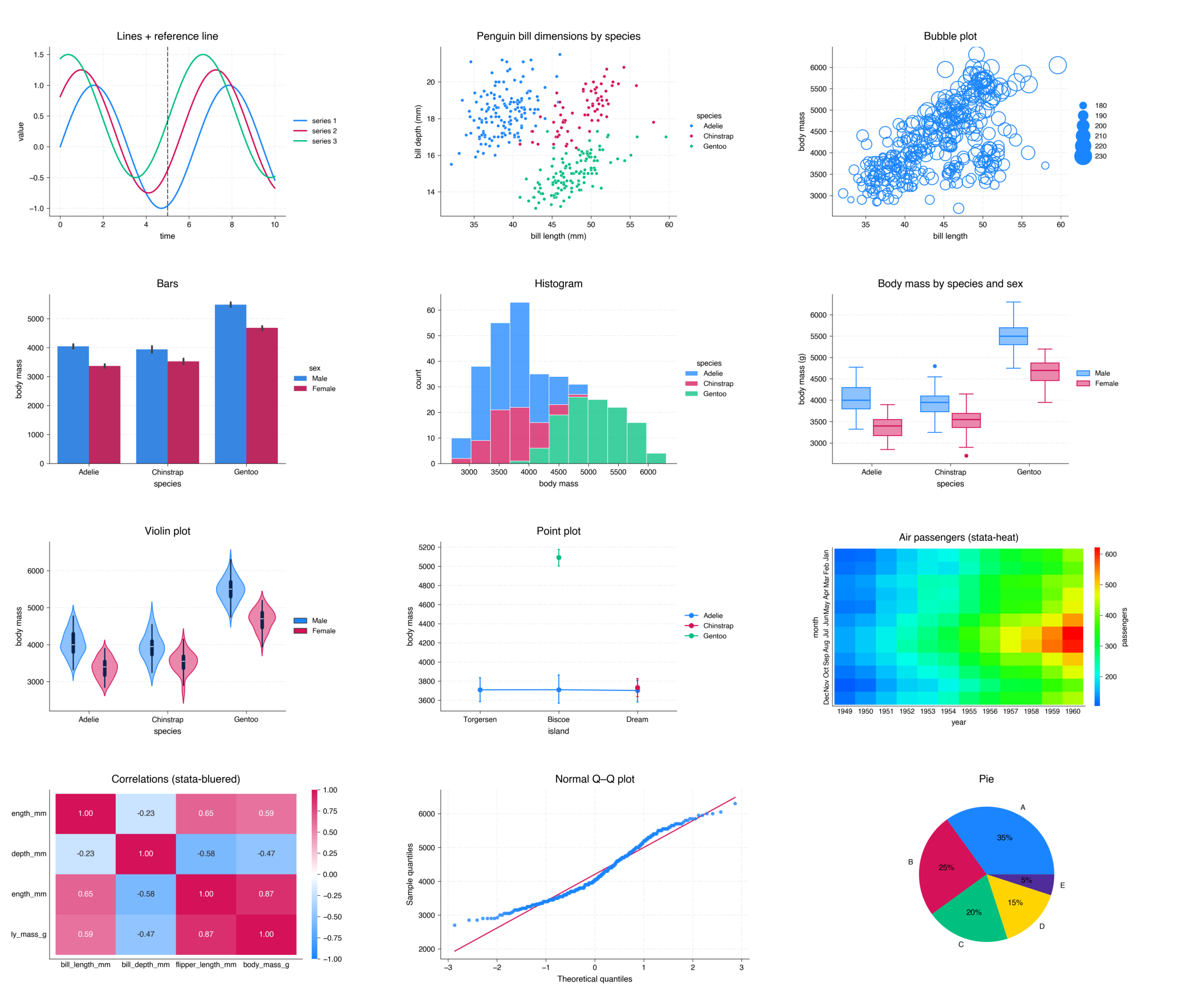
Give your matplotlib and seaborn charts the look of Stata 19
(the stcolor scheme, Stata's colorblind-friendly default). Calibrated against
the official SVG files exported by Stata 18/19.
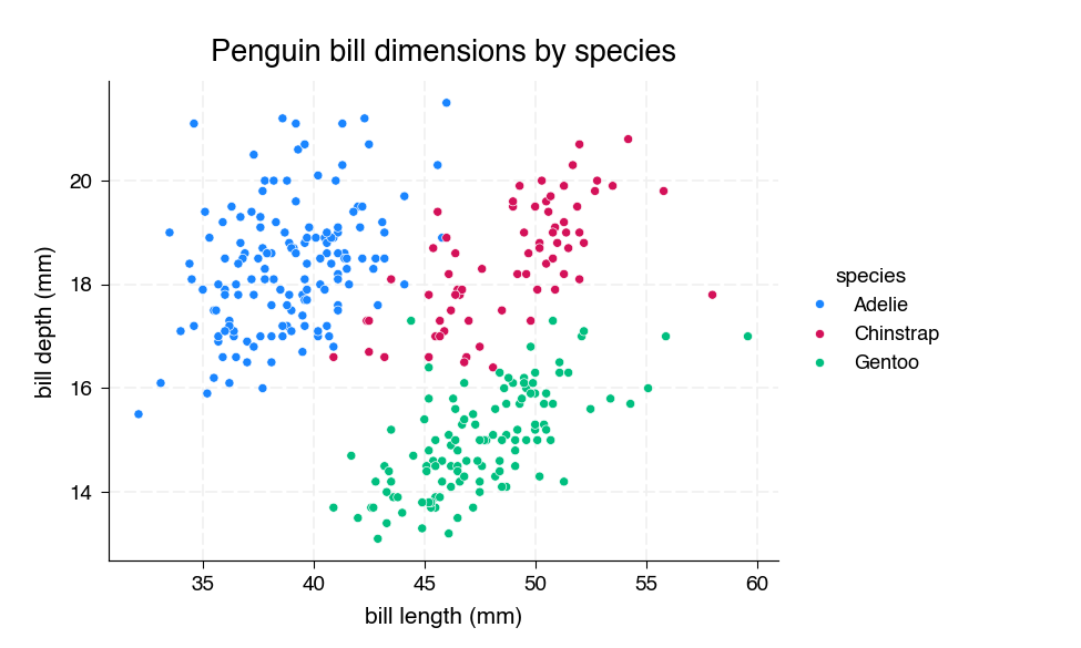
import seaborn as sns, stata_mpl

df = sns.load_dataset("penguins").dropna()

with stata_mpl.theme("scatter"):
    sns.scatterplot(df, x="bill_length_mm", y="bill_depth_mm", hue="species")
    # legend lands outside, to the right of the frame — like Stata
Nothing global is changed permanently: everything stays inside the with block.
Installation
cd stata-mpl
pip install -e .
Requires matplotlib>=3.4. For the seaborn integration: pip install -e ".[seaborn]"
(needs seaborn>=0.13).
seaborn — the recommended path
stata_mpl.theme() is a context manager that (1) applies the Stata style,
(2) sets the stcolor palette for seaborn — so you don't pass palette= for
hue — and (3) moves every legend outside, to the right of the frame, just
like Stata. No exceptions, for both seaborn and matplotlib legends.
import seaborn as sns, matplotlib.pyplot as plt, stata_mpl

df = sns.load_dataset("penguins").dropna()

with stata_mpl.theme("scatter"):
    fig, ax = plt.subplots()
    sns.scatterplot(df, x="bill_length_mm", y="bill_depth_mm", hue="species", ax=ax)
Stata-look seaborn wrappers
Seaborn draws box, violin and heatmap charts with its own artists, which ignore matplotlib's styling rcParams. The drop-in wrappers below reproduce Stata's per-group look (light fill + colored outline), add the heatmap gap, fix the jointplot zoom, draw hollow bubbles, and place the legend outside:
with stata_mpl.theme():
    stata_mpl.boxplot(df, x="species", y="body_mass_g", hue="sex")
    stata_mpl.violinplot(df, x="species", y="body_mass_g", hue="sex")
    stata_mpl.catplot(df, x="species", y="body_mass_g", hue="sex", kind="box")  # faceted
    stata_mpl.heatmap(flights_pivot)                       # native stata-heat
    stata_mpl.heatmap(df.corr(numeric_only=True), cmap="stata-bluered")  # correlations
    stata_mpl.jointplot(df, x="bill_length_mm", y="bill_depth_mm", hue="species")
    stata_mpl.residplot(df, x="bill_length_mm", y="body_mass_g")
    stata_mpl.bubbleplot(df, x="bill_length_mm", y="body_mass_g", size="flipper_length_mm")
    stata_mpl.pointplot(df, x="island", y="body_mass_g", hue="species")
    stata_mpl.qqplot(df["body_mass_g"])
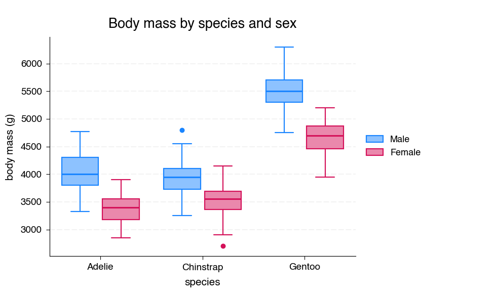
Each box/violin keeps the color seaborn assigned to its group — correct even
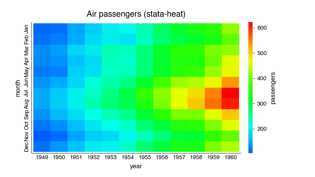
with unbalanced groups. The heatmap wrapper uses Stata's native multicolor
stata-heat map and leaves the small gap Stata draws around the cells:
Each wrapper accepts the same arguments as its sns.* counterpart and forwards
extra keyword arguments to it. Already have a seaborn axes you want to fix up?
Use stata_mpl.restyle_boxes(ax), restyle_violins(ax) or add_heatmap_gap(ax).
matplotlib — the style-context path
You can also stack a base style with a chart-type overlay through matplotlib's own style context (no seaborn required):
import numpy as np, matplotlib.pyplot as plt, stata_mpl

x = np.linspace(0, 10, 200)
with plt.style.context(["stata", "line"]):
    fig, ax = plt.subplots()
    ax.plot(x, np.sin(x), label="sin")
    ax.plot(x, np.cos(x), label="cos")
    ax.set(title="Example", xlabel="time", ylabel="value")
    stata_mpl.legend(ax)          # legend outside, right of the frame
stata_mpl.theme("line") is the same thing plus the automatic outside legend.
Available styles
The base style carries the overall look (white background, 7.5×4.5" figure,
balanced margins, long-dashed horizontal grid #F0F0F0, thin black axes,
stcolor palette, borderless legend, enlarged titles). Chart-type overlays
stack on top.
| Style | Chart type | Specifics |
|---|---|---|
stata |
base (Stata 19 default) | stcolor palette, grid, axes, margins, font |
stata-classic |
base (s2color scheme) |
historical palette, solid grid |
boxplot |
ax.boxplot |
#8DC2FF boxes, stc1 outline/median |
scatter |
ax.scatter / sns.scatterplot |
small filled markers, grid on both axes |
line |
ax.plot / sns.lineplot |
solid curves, no markers, grid on both axes |
histogram (hist) |
ax.hist / sns.histplot |
stc1 bars, bins=auto |
bar |
ax.bar / sns.barplot |
solid bars, no seam (like Stata) |
violin |
ax.violinplot / sns.violinplot |
horizontal grid, palette colors |
errorbar |
ax.errorbar |
caps + point estimate, grid on both axes |
area |
stackplot / fill_between |
stcolor areas |
pie |
ax.pie |
no axes, no grid |
heatmap |
imshow / contourf / sns.heatmap |
no grid, native stata-heat cmap, cell gap |
Each overlay also has a prefixed alias (stata-boxplot…) to avoid name clashes.
Chart-type coverage
All common types are covered (see examples/coverage_check.py, which exercises
47): matplotlib (line, scatter, bar/barh, hist, box, violin, errorbar,
stackplot, pie, imshow, hexbin, step, stem, contourf, quiver) and seaborn
(scatter/line/hist/kde/box/violin/bar/strip/swarm/point, regplot, residplot,
lmplot, catplot, jointplot, JointGrid, pairplot, displot, relplot, heatmap),
plus qqplot (statsmodels / scipy.stats.probplot).
Palette & colormaps
stata_mpl.PALETTE          # ['#1A85FF', '#D41159', '#00BF7F', ...]  (15 stcolor colors)
stata_mpl.palette(3)       # first 3, in order
stata_mpl.COLORS           # {'stblue': '#1A85FF', 'stred': '#D41159', 'navy': '#08234C', ...}
stata_mpl.lighten("#1A85FF")  # -> light-blue box fill (#8DC2FF); 50% toward white
Registered colormaps (for cmap=...), on top of native viridis/plasma:
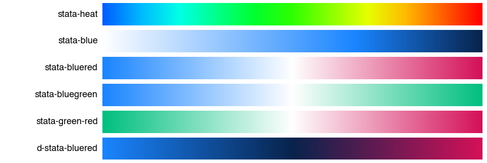
| Colormap | Type | Use |
|---|---|---|
stcolor |
discrete | 15 categorical colors |
stata-heat |
multicolor | Stata's native heatmap/imshow rainbow |
stata-blue |
sequential | heatmaps (white → navy) |
stata-bluered |
diverging | correlations (blue → white → red) |
stata-bluegreen |
diverging | blue → white → green |
stata-green-red |
diverging | green → white → red |
d-stata-bluered |
diverging | dark-center (blue → navy → red) |
(reversed …_r variants are available too). stata-heat is applied
automatically to imshow / contourf / pcolormesh under the heatmap
overlay, and is the default for stata_mpl.heatmap().
Reference lines
Inside theme(), ax.axvline / ax.axhline automatically take the Stata
reference-line look — the grid's dash pattern, but black — unless you pass your
own color / linestyle / linewidth:
with stata_mpl.theme("line"):
    fig, ax = plt.subplots()
    ax.plot(years, y)
    ax.axvline(2018)                 # grid dashes, black
    stata_mpl.refline(ax, y=0)       # same, usable outside theme() too
stata_mpl.residplot() draws seaborn's residual plot with its y=0 baseline in
that same style.
Grids
Charts whose both axes are continuous (scatter, line, bubble, jointplot,
Q–Q…) show the grid on both axes, like Stata. Categorical charts (bar, box,
violin, histogram) keep the horizontal grid only. To override on a given axes:
ax.grid(axis="y") or ax.grid(axis="both").
Annotations
stata_mpl.label_points(ax, x, y, labels) writes Stata-style marker labels — in
the marker's color, next to each point (position= is "right"/"left"/"top"
/"bottom").
Helpers
stata_mpl.theme(chart=None)— context manager: Stata style + outside-right legends + grid-black reference lines + seaborn palette. The recommended entry point.stata_mpl.legend(ax)— borderless legend outside, right of the frame, with the plotting area shrunk so nothing is clipped.stata_mpl.refline(ax, x=, y=)— reference line with the grid look, in black.stata_mpl.label_points(ax, x, y, labels)— Stata marker labels (marker color).stata_mpl.boxplot / violinplot / catplot— box/violin (incl. facets) with the per-group Stata look.stata_mpl.bubbleplot / pointplot— hollow-circle bubbles / capped point estimates.stata_mpl.heatmap / jointplot / residplot / qqplot— Stata heatmap, de-zoomed joint, grid-black residual baseline, stcolor Q–Q.stata_mpl.lighten(color)— blend a color 50 % toward white (Stata box fill).stata_mpl.set_palette()/palette(n)— stcolor palette for seaborn.stata_mpl.notebook_setup()— keep Stata margins in Jupyter's inline display.
Examples
examples/examples.ipynb— full tutorial notebook covering every chart type.examples/gallery.py— gallery of the main chart types (examples/output/gallery.png).examples/coverage_check.py— verifies coverage of all 47 chart types.
In Jupyter (margins)
The style controls savefig (exported PNGs keep the right margins), but inline
display crops by default. To keep the wide Stata margins:
stata_mpl.notebook_setup() # or: %config InlineBackend.print_figure_kwargs = {"bbox_inches": None}
Known limitations
- Area transparency:
fill_between/stackplothave no opacity rcParam → passalpha=...at call time. barh: thebaroverlay puts the grid on the y axis; for horizontal bars addax.grid(axis="x").- seaborn figure-level (
lmplot,catplot,relplot,displot,pairplot): they manage their own figure; size them viaheight/aspect. Thejointplotwrapper handles the layout and legend for you. - The box/violin restyling targets seaborn ≥ 0.13; on other versions the chart still renders (it simply falls back to seaborn's default colors).
License
MIT — see LICENSE. © 2026 Lucas Duthu.
This is free, community-developed open-source software.
Disclaimer
stata-mpl is an independent, unofficial open-source project. It is not affiliated with, endorsed by, sponsored by, or connected to StataCorp LLC.
"Stata" and "stcolor" are trademarks or product names of StataCorp LLC. They are used here in a purely descriptive, nominative way: stata-mpl reproduces the visual appearance of Stata's default graph scheme so that matplotlib/seaborn figures look familiar to Stata users. The project ships no StataCorp code, data, or assets — the colors and layouts were re-derived independently from publicly visible chart output. If you represent StataCorp and have any concern, please open an issue.
Release history Release notifications | RSS feed

Download files
Download the file for your platform. If you're not sure which to choose, learn more about installing packages.
Source Distribution
Built Distribution
Filter files by name, interpreter, ABI, and platform.
If you're not sure about the file name format, learn more about wheel file names.
Copy a direct link to the current filters
File details
Details for the file stata_mpl-0.3.0.tar.gz.
File metadata
- Download URL: stata_mpl-0.3.0.tar.gz
- Upload date:
- Size: 1.3 MB
- Tags: Source
- Uploaded using Trusted Publishing? No
- Uploaded via: twine/6.2.0 CPython/3.13.5
File hashes
| Algorithm | Hash digest | |
|---|---|---|
| SHA256 |
1d22102712beb7585760e8459b15700961b1f42bedc84f710bedb49b5a16e941
|
|
| MD5 |
95614bafb1643bae4650ff35b459eb9f
|
|
| BLAKE2b-256 |
a4380e0fc1e39725a6f5eb38bc9276ab6b0a90e2bf4410eb1955c62c7078f247
|
File details
Details for the file stata_mpl-0.3.0-py3-none-any.whl.
File metadata
- Download URL: stata_mpl-0.3.0-py3-none-any.whl
- Upload date:
- Size: 25.7 kB
- Tags: Python 3
- Uploaded using Trusted Publishing? No
- Uploaded via: twine/6.2.0 CPython/3.13.5
File hashes
| Algorithm | Hash digest | |
|---|---|---|
| SHA256 |
7c6f8caa46ad6a3e72aa880f94dede63fb983559d0ff7daf6b1402971b5b8dd2
|
|
| MD5 |
322af8a53990c244ac7ad4ae2044d43c
|
|
| BLAKE2b-256 |
5bd3e95650fa40846cfcf2bdb88a7f1997878e9dca815c854d7518c1cffaf76d
|






