
A Python helper library for generating Process Behaviour Charts
Verified details
These details have been verified by PyPIProject links
GitHub Statistics
Maintainers

Project description
statprocon
statprocon is a Python helper library for generating data for use in Statistical Process Control charts. SPC charts are also known as Process Behaviour Charts, Control charts or Shewhart charts.
SPC Charts help answer questions like:
- How do I know a change has occurred in a process?
- What is the expected variation in a process?
- Is a process stable or unpredictable?
Installation
pip install statprocon
To use the built-in plotting helpers (x_plot() / mr_plot()), install the optional plot extra,
which pulls in matplotlib and pandas:
pip install statprocon[plot]
Usage
from statprocon import XmR

counts = [10, 50, 40, 30]

xmr = XmR(counts)
moving_ranges = xmr.moving_ranges()
unpl = xmr.upper_natural_process_limit()[0]  # 85.7
lnpl = xmr.lower_natural_process_limit()[0]  # -20.7
x_cl = xmr.x_central_line()[0]  # 32.5

url = xmr.upper_range_limit()[0]  # 65.36
mr_cl = xmr.mr_central_line()[0]  # 20
Currently, this library only supports the data for generating an XmR chart. An XmR chart is the most universal way of using process behaviour charts. XmR is short for individual values (X) and a moving range (mR). More chart data options can be added via pull requests.
For more information, please read Making Sense of Data by Donald Wheeler.
pandas
Visualize XmR charts using Jupyter Notebooks and pandas
import pandas as pd
from statprocon import XmR

xmr = XmR(counts)

pd.DataFrame(xmr.x_to_dict()).astype(float).plot()
pd.DataFrame(xmr.mr_to_dict()).astype(float).plot()

Charts can display X-axis labels by using the following code:
labels = ['0', '1', '2', '3']
pd.DataFrame(xmr.x_to_dict(), index=labels).astype(float).plot()
Or use built-in methods to generate charts that highlight detection points.
These require the optional plotting dependencies (pip install statprocon[plot]):
labels = ['J', 'F', 'M', ...]
xmr = XmR(counts)
xmr.x_plot(labels)
xmr.mr_plot(labels)
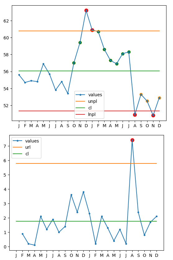
Data points that meet detection rules are marked by the following colours:
| Rule | Colour |
|---|---|
| Rule 1 | Red |
| Rule 2 | Green |
| Rule 3 | Orange |
If one data point meets the criteria for multiple detection rules, the lower numbered detection rule will take priority and be marked. For example, if a data point meets all detection rules, it will be displayed in red. If a data point meets rule 2 and rule 3, it will be displayed in green.
CSV
Generate a CSV of all the data needed to create XmR charts.
print(xmr.to_csv())
Google Sheets Charts
Generate XmR Charts in Google Sheets
https://github.com/mattmccormick/statprocon/assets/436801/0de1a9f3-a8ad-4047-8c9d-0f890e0bf453
- Make a copy of the statprocon XmR Template sheet
- Paste the CSV output from above into cell A1
- Click
Data -> Split Text to Columns
The X and MR charts will appear on the right.
Note that the Lower Natural Process Limit may not make sense if your count data could not possibly go negative. If LNPL is not needed, remove it with the following steps:
- Double-click on the X Chart
- Click the
Setuptab - Under
Series, findLNPL - Click the 3 dot menu on the right next to
LNPL - Click
Remove
The LNPL line will be removed from the X Chart.
Advanced Usage
Halfway Lines
Halfway lines between the X central line and the Upper and Lower Natural Process Limits can be returned by using the include_halfway_lines argument:
xmr.x_to_dict(include_halfway_lines=True)
When the process is predictable, approximately 85% of the X values fall between the Upper and Lower halfway lines.
Trending Limits
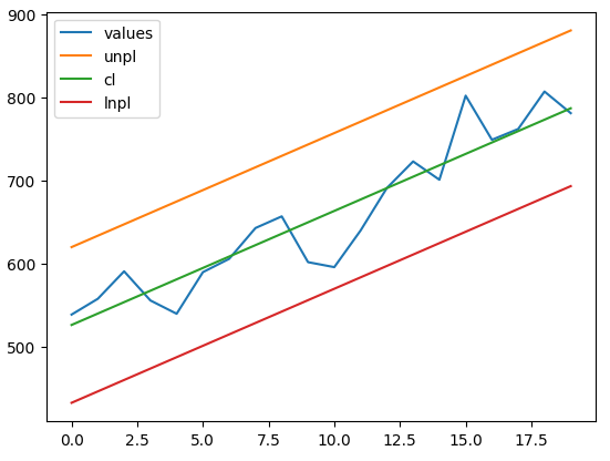
With data points that trend upwards or downwards over time, use Trending Limits to calculate a sloping X central line, Upper Natural Process Limits and Lower Natural Process Limits.
from statprocon import XmRTrending

counts = [...]  # data from TrendingTestCase.test_trending_limits

source = XmR(counts)
trending = XmRTrending(source)
pd.DataFrame(trending.x_to_dict()).astype(float).plot()
Use the Median Moving Range
If your data contains extreme outliers, it may be better to compute the limits using the median moving range.
xmr = XmR(counts, moving_range_uses='median')
Use the Median for the X Central Line
xmr = XmR(counts, x_central_line_uses='median')
Note: It's assumed that by using the median for the X central line that the median moving range should also be used. For example, you cannot do the following:
xmr = XmR(counts, x_central_line_uses='median', moving_range_uses='average')
Calculate Limits from Subset of Counts
The central lines and limits calculations can be restricted to a subset of the count data.
Use the subset_start_index and subset_end_index parameters when instantiating the XmR object:
xmr = XmR(counts, subset_start_index=10, subset_end_index=34) # 24 points of data starting at index 10
When one or both of these optional arguments are provided, the the X and MR central line calculations will be modified to only use the data from subset_start_index up to, but not including, subset_end_index.
When these optional arguments are not provided, subset_start_index defaults to 0 and subset_end_index defaults to the length of counts.
Dependencies
There are a few other Python libraries for generating SPC charts but they all contain large dependencies in order to include the ability to graph the chart.
This package will remain small and light: the core package has no required dependencies, and the data can be converted into charts on your own.
The plotting helpers (x_plot() / mr_plot()) are optional and only pull in matplotlib and pandas when you install the plot extra (pip install statprocon[plot]).
This package also contains extensive tests for verifying the integrity of the calculated data.
Development
This project uses uv for dependency management and packaging. Install it by following the installation guide.
Create the virtual environment and install all dependencies (including dev tools):
uv sync
To build the distribution locally:
uv build
Releasing
Releases are published to PyPI automatically by the release workflow when a version tag is pushed:
-
Bump
versioninpyproject.tomland add a matching section toCHANGELOG.md. -
Merge to
main. -
Tag the release and push the tag:
git tag v2.0.1
git push origin v2.0.1
The workflow verifies the tag matches the package version, builds the
distribution, publishes to PyPI via trusted publishing
(no API tokens), and creates a GitHub Release from the CHANGELOG entry.
Publishing waits for manual approval on the protected pypi environment.
Testing
Run tests
uv run python -m unittest discover
Run type checking
uv run mypy statprocon tests
Project details
Verified details
These details have been verified by PyPIProject links
GitHub Statistics
Maintainers
Release history Release notifications | RSS feed


Download files
Download the file for your platform. If you're not sure which to choose, learn more about installing packages.
Source Distribution
Built Distribution
Filter files by name, interpreter, ABI, and platform.
If you're not sure about the file name format, learn more about wheel file names.
Copy a direct link to the current filters
File details
Details for the file statprocon-2.0.0.tar.gz.
File metadata
- Download URL: statprocon-2.0.0.tar.gz
- Upload date:
- Size: 111.0 kB
- Tags: Source
- Uploaded using Trusted Publishing? Yes
- Uploaded via: uv/0.11.18 {"installer":{"name":"uv","version":"0.11.18","subcommand":["publish"]},"python":null,"implementation":{"name":null,"version":null},"distro":{"name":"Ubuntu","version":"24.04","id":"noble","libc":null},"system":{"name":null,"release":null},"cpu":null,"openssl_version":null,"setuptools_version":null,"rustc_version":null,"ci":true}
File hashes
| Algorithm | Hash digest | |
|---|---|---|
| SHA256 |
88477e525834451b0a662aff97235c64b453814059aa4b74327fc8e1e24dd6d6
|
|
| MD5 |
9d9b11147cd79361adc24659ac3abcd1
|
|
| BLAKE2b-256 |
f81dd8e53f5fcae4763fafee1a3be58968a411fe63491ccdf49902a0848766f0
|
File details
Details for the file statprocon-2.0.0-py3-none-any.whl.
File metadata
- Download URL: statprocon-2.0.0-py3-none-any.whl
- Upload date:
- Size: 13.0 kB
- Tags: Python 3
- Uploaded using Trusted Publishing? Yes
- Uploaded via: uv/0.11.18 {"installer":{"name":"uv","version":"0.11.18","subcommand":["publish"]},"python":null,"implementation":{"name":null,"version":null},"distro":{"name":"Ubuntu","version":"24.04","id":"noble","libc":null},"system":{"name":null,"release":null},"cpu":null,"openssl_version":null,"setuptools_version":null,"rustc_version":null,"ci":true}
File hashes
| Algorithm | Hash digest | |
|---|---|---|
| SHA256 |
fda12de212bd8cda98fe8b96f77ca4616770ab9c49c33172372cbde6451299eb
|
|
| MD5 |
f99e234e1d0246ecdb592433f85a93eb
|
|
| BLAKE2b-256 |
44f8e51cf6a669352ecc96485859ade5f85a7b1b35e0eb950e2e16abf3566814
|






