
Matrix decomposition of neurophysiological event waveform populations

Project description
subwave
Data-driven decomposition of neurophysiological event waveform populations.
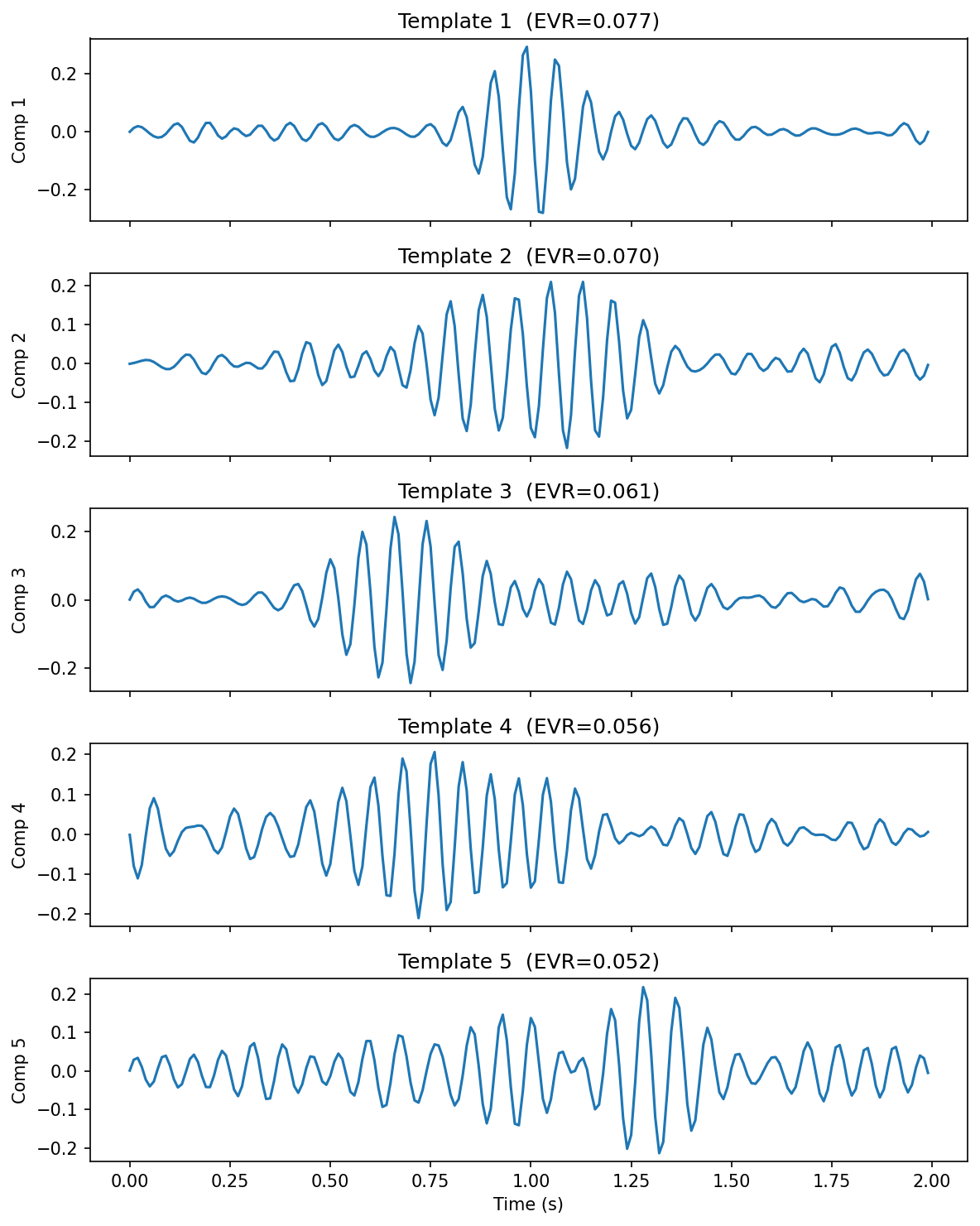
Five principal waveform templates extracted from 821 sleep spindles via SVD.
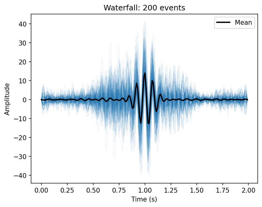
200 sigma-filtered spindle waveforms overlaid, with the population mean in black.
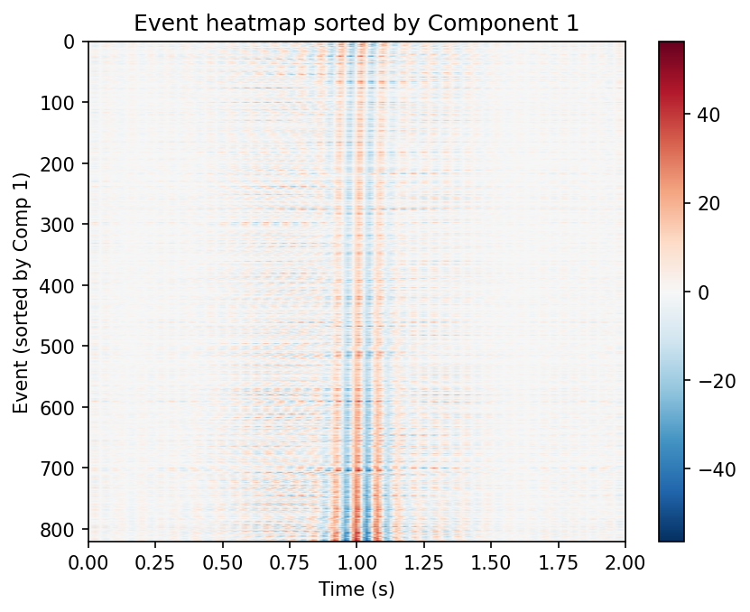
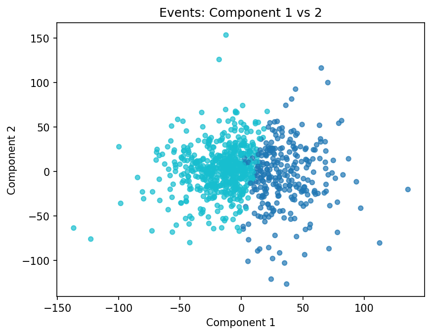
Left: all events sorted by Component 1 loading. Right: k-means clustering in the first two component scores.
Install
pip install subwave
Optional extras:
pip install "subwave[mne]"          # MNE-Python and Luna I/O
pip install "subwave[yasa]"         # YASA spindle detection I/O (pulls in mne)
pip install "subwave[scattering]"   # Wavelet scattering decomposition (kymatio)
pip install "subwave[tensor]"       # Multi-channel tensor decomposition (tensorly)
pip install "subwave[all]"          # All optional backends
Quickstart
import numpy as np
import subwave as sw

rng = np.random.default_rng(0)
t = np.linspace(0, 1, 256)
X = np.stack([np.sin(2 * np.pi * 13 * t) + rng.normal(0, 0.1, 256) for _ in range(100)])

result = sw.decompose(X, method="svd", n_components=5)
result.plot_templates(n=3)
Each template is a basis waveform shape; each loading is how strongly a given event expresses that template. Together they reconstruct the original population.
Or let subwave choose the number of components:
result = sw.decompose(X, n_components="auto")
ECG example
import numpy as np
import subwave as sw

# Stack detected QRS complexes into an event matrix
X_beats = np.load("heartbeats.npy")     # (n_beats, n_samples)
result = sw.decompose(X_beats, method="svd", n_components=3)

# Outlier detection flags ectopic beats
scores = result.outlier_scores()
ectopic = np.where(scores > np.percentile(scores, 99))[0]
Loading data
sw.from_array(X, sfreq=256)                              # plain numpy
sw.from_npz("spindles.npz")                              # Lunascope format
sw.from_mne(epochs)                                       # MNE Epochs
sw.from_yasa(spindles_df, raw_signal, sfreq=256)          # YASA output
sw.from_luna("spindles.txt", "recording.edf", sfreq=256)  # Luna output + EDF
sw.from_edf_batch(["s1.edf", "s2.edf"], channel="C3")     # detect + pool across files
sw.from_lwf("spindles.lwf")                               # Luna .lwf waveform export
from_edf_batch runs a detector (default YASA) on every EDF, extracts windows
around each peak, and returns a single EventMatrix with a .meta DataFrame
recording subject, file, event_index, and peak_sec for each pooled
event.
Luna .lwf files
from_lwf reads Luna's binary .lwf waveform export directly (no optional
dependencies required) and returns an AxisAnnotatedTensor with axes
['instance', 'channel', 'sample'], preserving per-channel labels/units/sample
rates and rich per-event metadata (annotation, instance, anchor and timing
columns):
aat = sw.from_lwf("spindles.lwf")          # a single file
aat = sw.from_lwf(["s1.lwf", "s2.lwf"])    # several files, concatenated
aat = sw.from_lwf("exports/", recur=True)  # every .lwf under a directory

aat.shape                                  # (n_events, n_channels, n_samples)
aat.axis_meta["instance"]                  # per-event DataFrame (id, annot, timing, …)
aat.axis_meta["channel"]                   # label, unit, sr per channel
result = sw.decompose(aat, method="svd", n_components=5)
All files must share the same channel labels and sample rates, and every event
must have the same number of samples (Luna's require=full windows). To inspect
files without loading any signal data, use lwf_summary:
df = sw.lwf_summary("exports/", recur=True)
# One row per file: id, tag, startdate, n_waves, n_channels, channels, srs, …
Decomposition methods
- SVD / PCA (
method='svd') — default, optimal low-rank approximation. Uses randomized SVD for >5000 events. - NMF (
method='nmf') — parts-based, requires non-negative input. - Dictionary learning (
method='dictlearn') — sparse atoms. - Fourier-then-SVD (
method='fourier_svd') — shift-invariant: SVD on per-event magnitude rFFT spectra. Robust to small temporal jitter that corrupts plain SVD. Templates live in frequency space (config['domain'] = 'frequency'). - Scattering-then-SVD (
method='scattering_svd') — locally translation-invariant and stable to deformation via 1-D wavelet scattering (kymatio). Templates live in scattering-coefficient space. Requiressubwave[scattering].
Tensor decomposition (multi-channel)
For 3-D event tensors (n_events, n_samples, n_channels), tensor_decompose
factors temporal and spatial structure separately instead of flattening:
result = sw.tensor_decompose(X, method="cp", rank=3)        # PARAFAC / CP
result = sw.tensor_decompose(X, method="tucker", rank=3)    # Tucker (with core)

result.event_factors        # (n_events, rank)
result.temporal_factors     # (n_samples, rank)
result.spatial_factors      # (n_channels, rank)
result.reconstruction_error # ||X - X_hat|| / ||X||
result.component_waveform(0, channel=1)   # template scaled by channel weight
result.plot()                             # per-component temporal / spatial / loading panels
Requires subwave[tensor].
Working with results
result.templates                        # (n_components, n_samples) basis waveforms
result.loadings                         # (n_events, n_components) per-event scores
result.explained_variance_ratio         # variance captured per component
result.singular_values                  # singular values
result.factor_tables["instance"]        # DataFrame: instance_id, score_1…k, recon_error

result.reconstruct(n_components=3)      # rank-k reconstruction
result.project(new_X)                   # project new events onto learned subspace
result.outlier_scores()                 # per-event reconstruction error
Component selection
k = sw.parallel_analysis(X)             # Horn's parallel analysis
k = sw.elbow(result.singular_values)    # Kneedle elbow detection
k = sw.kaiser(result)                   # Kaiser rule
Spectral characterization
freqs, powers = result.template_spectrum(sfreq=256)
peak_hz = result.template_peak_freq(sfreq=256)     # e.g. [13.2, 11.1] Hz
bw_hz = result.template_bandwidth(sfreq=256)
Clustering
cr = result.cluster(method="kmeans", n_clusters=2)
cr["labels"]                            # cluster assignments
result.cluster_templates(n_clusters=2)  # mean waveform per cluster
Group comparison
perm = sw.permutation_test(X, groups, n_components=3, n_perm=500)
perm.p_value                            # do two groups span different subspaces?

df = sw.comparison.loading_test(result, groups, n_perm=1000)
# Columns: component, observed_diff, p_value, cohens_d, p_corrected
# cohens_d:    standardized effect size (pooled SD)
# p_corrected: Benjamini-Hochberg FDR-adjusted p-values across components
Spindle helpers
Convenience routines for sleep-spindle waveforms (sigma-band filtering, envelope-based alignment, canonical templates).
from subwave.spindles import (
    sigma_filter,             # 9–16 Hz Butterworth bandpass (sosfiltfilt)
    align_by_envelope_peak,   # circularly shift so each event's sigma-envelope peak is centered
    CANONICAL_FAST,           # ~13.5 Hz Gaussian-windowed sinusoid (256 Hz, 1 s)
    CANONICAL_SLOW,           # ~11 Hz   Gaussian-windowed sinusoid (256 Hz, 1 s)
)

X_filt = sigma_filter(X, sfreq=256)
X_aligned = align_by_envelope_peak(X, sfreq=256)
Validation
Tools for checking decompositions against ground truth and for estimating component reliability.
from subwave.validation import (
    synthetic_population,   # generate events from known templates with noise / jitter / amplitude variability
    recovery_score,         # cosine similarity between true and recovered templates (Hungarian-matched)
    cluster_recovery_ari,   # Adjusted Rand Index between true and recovered cluster labels
    bootstrap_stability,    # mean cosine similarity of bootstrap-resampled templates to full-data templates
    split_half,             # template & loading reproducibility on odd/even split
)

# Ground-truth recovery on synthetic data
truth = synthetic_population(templates, n_events=200, noise_std=0.1, random_state=0)
result = sw.decompose(truth["X"], method="svd", n_components=truth["templates"].shape[0])
score = recovery_score(truth["templates"], result.templates)
score["mean_score"]            # cosine similarity (1.0 = perfect)

# Reliability of a real decomposition
boot = bootstrap_stability(X, n_components=3, n_boot=100, random_state=0)
boot["stability_scores"]       # per-component mean similarity across bootstraps

sh = split_half(X, n_components=3, random_state=0)
sh["template_similarity"]      # per-component template reproducibility
sh["loading_correlation"]      # correlation of projected vs native loadings
Serialization
result.save("result.npz")
result = sw.load_result("result.npz")
df = result.to_dataframe()              # flat DataFrame for R/Stata
Plots
result.plot_spectrum()                  # singular value scree plot
result.plot_templates(n=5)              # basis waveforms
result.plot_template_spectra(sfreq=256) # power spectrum of each template
result.plot_scatter(x=0, y=1)           # component 0 vs 1 (supports color= for clusters)
result.plot_heatmap(comp=0)             # events × samples sorted by loading
result.plot_waterfall(n=100)            # overlaid waveforms with bold mean
result.plot_mean_pm(comp=0)             # mean ± component
result.plot_sorted_grid(comp=0)         # events sorted by score
result.plot_residual_hist()             # reconstruction error distribution
result.plot_cumulative_variance()       # cumulative EVR curve
result.plot_reconstruction(event_idx=0) # original vs reconstruction
result.plot_loadings_by_group(groups)   # box/violin by group
result.plot_loadings_over_time(times)   # loading drift across time
See docstrings via help(sw.decompose) for full options, including cluster_sweep, loading_test, subspace_angles, scatter_colored_by, loadings_correlated_with, and more.
Citation
If you use subwave in published work, see CITATION.cff in the repository.
License
MIT


Download files
Download the file for your platform. If you're not sure which to choose, learn more about installing packages.
Source Distribution
Built Distribution
Filter files by name, interpreter, ABI, and platform.
If you're not sure about the file name format, learn more about wheel file names.
Copy a direct link to the current filters
File details
Details for the file subwave-0.3.0.tar.gz.
File metadata
- Download URL: subwave-0.3.0.tar.gz
- Upload date:
- Size: 1.1 MB
- Tags: Source
- Uploaded using Trusted Publishing? No
- Uploaded via: twine/6.2.0 CPython/3.14.0
File hashes
| Algorithm | Hash digest | |
|---|---|---|
| SHA256 |
095e0836b3be3c85371964143a0a12b18b704e8c915e002d4eb8cf1e9fa60640
|
|
| MD5 |
50291e54bcc5184f4663275158ffe4c0
|
|
| BLAKE2b-256 |
32394f75b2c74bc4e2de9848d4ece4d5a3aed087d7cbb2ee61af3fb01c2c0deb
|
File details
Details for the file subwave-0.3.0-py3-none-any.whl.
File metadata
- Download URL: subwave-0.3.0-py3-none-any.whl
- Upload date:
- Size: 45.4 kB
- Tags: Python 3
- Uploaded using Trusted Publishing? No
- Uploaded via: twine/6.2.0 CPython/3.14.0
File hashes
| Algorithm | Hash digest | |
|---|---|---|
| SHA256 |
316ceb4e08102e247785ae3c3bccf5ac1b6d7c1ef012075d50697d53f785f38f
|
|
| MD5 |
35aa72f26ba7904e0ee63f412eb9e358
|
|
| BLAKE2b-256 |
1d264e4d3b72ad8d5b3b3e5a4367c8df7c1a175d9b8b3101f1b6c292b22a7050
|






