
Shallow Water Equations Solver
This package provides a well-balanced solver for the one-dimensional Saint-Venant equations, based on the principles outlined in this paper and this presentation.
Installation
The package is available through pip, and may be installed via:
pip install SWE_Solver
Main Usage
To utilize this package, you can call the plotSWE function with the following parameters:
h, u = plotSWE(B, h0, u0, Nx, tEnd, timePoints, g=1, method='C')
Parameters:
- B (callable): Bottom topography function. This function defines the topographic profile and should take spatial coordinates as input and return the bottom elevation at those coordinates.
- h0 (array): Initial water height profile. This should be an array of length
Nx, representing the initial water height at different spatial locations. - u0 (array): Initial water velocity profile. Similar to h0, this should be an array of length
Nx, representing the initial water velocity at different spatial locations. - Nx (int): Number of spatial grid points.
- tEnd (float): End time of the simulation. The simulation starts at time t=0.
- timePoints (list): List of time points at which you want to visualize the results.
- g (float, optional): Gravitational constant. Default is
1. - method (str, optional): Method selection (
'A','B'or'C'). Default is'C'.
Returns:
- h (array): Array containing the water height profile at the final time point.
- u (array): Array containing the water velocity profile at the final time point.
Pre-Coded Examples
A number of pre-coded examples are available through the library, through the function exampleSWE.
h, u = exampleSWE(state="still_flat", method='C')
Parameters
- state (String): Name of the example. Has to be one of
"still_flat"(Constant height, zero velocity, flat bottom),"still_tilted"(Constant total height, zero velocity, tilted bottom),,"still_tilted_pert"(Perturbed constant total height, perturbed zero velocity, tilted bottom),"moving_flat"(Constant height, constant velocity, flat bottom),"moving_tilted"(Constant total height, constant velocity, tilted bottom),"evolving_wave"(Step function for height, constant discharge, flat bottom),"standing_wave"(Final profile of"evolving_wave"for method'C', representing an equilibrium),"standing_wave_pert"(Final profile of"evolving_wave"for method'C', with a perturbation),"forming_collision"(Constant water height, positive velocity on the right, negative velocity on the left, flat bottom),"spike_flattening"(Water height given by a Gaussian, zero velocity, flat bottom),"over_bump"(Constant total water height, constant velocity, bottom given by a Gaussian). Defaults to"still_flat". - method (String): Name of the method used. Has to be one of
'A','B','C'. Defaults to'C'.
Returns
- h (array): Array containing the water height profile at the final time point.
- u (array): Array containing the water velocity profile at the final time point.
Example
from SWE_Solver import plotSWE
from math import sqrt
from scipy.special import erf

Nx = 50
B = lambda x: 1
f = lambda T: 1 + sqrt(3) / (1 - erf(-0.5 / 0.1)) * (erf((T - 0.5) / 0.1) - erf (-0.5 / 0.1))
h0 = [f(_/ (Nx-1)) for _ in range(Nx)]
u0 = [2.0 / h0[_] for _ in range(Nx)]
_ = plotSWE(B, h0, u0, Nx, tEnd=1.0, timePoints=[0.0, 0.1, 0.5, 1.0])
The above is equivalent to the simple example given by
from SWE_Solver import exampleSWE

_ = exampleSWE("evolving_wave", 'C')
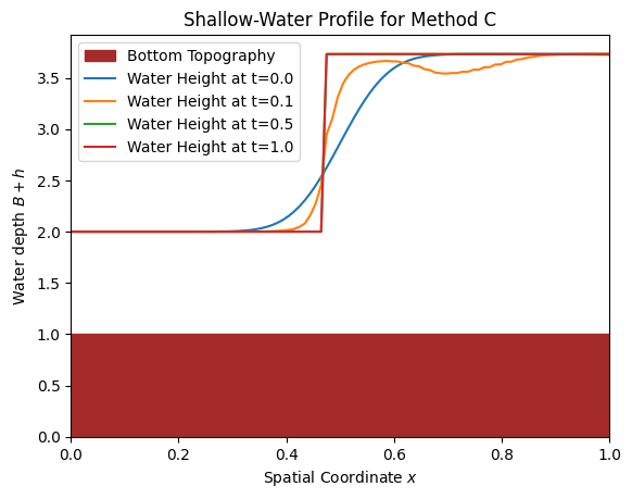
In this example, we're using a spatial grid with 50 points, running the simulation up to t=1 seconds, and visualizing the results at times 0.0, 0.1, 0.5 and 1.0 seconds, with gravitational constant g=1 (default value) and using method='C' (default value).
This produces the result in the following figure.
1 maintainer

Metadata
1 maintainer
Release files for SWE-Solver 0.1.7
For a detailed explanation of source distributions (sdists) and built distributions (wheels), please see the package formats documentation.
Source distribution (sdist)
| File | Size | Uploaded | |
|---|---|---|---|
| SWE_Solver-0.1.7.tar.gz | 14.7 kB | Details |
Built distribution (wheel)
| File | Interpreter | ABI | Platform | Reset |
|---|---|---|---|---|
| SWE_Solver-0.1.7-py3-none-any.whl | Python 3 | none | any | Details |
Total release size: 29.3 kB
Release files / SWE_Solver-0.1.7.tar.gz
| Download URL | SWE_Solver-0.1.7.tar.gz |
|---|---|
| Size | 14.7 kB |
| Tags | Source |
|
SHA-256 checksum How to use checksums |
21c7aeeb80cb11cd42602b4edf487eb37053db17d61999088de3b48691f43ed8
|
|
BLAKE2b-256 checksum How to use checksums |
7cc6a057df7d36654fa2ebc27c017fbd9a107dcff67ece9ccdcecf50df75e2e5
|
| Upload date | |
|
Uploaded using Trusted Publishing? What is trusted publishing? |
No |
| Uploaded via |
twine/4.0.2 CPython/3.11.5
|
Release files / SWE_Solver-0.1.7-py3-none-any.whl
| Download URL | SWE_Solver-0.1.7-py3-none-any.whl |
|---|---|
| Size | 14.6 kB |
| Tags | Python 3 |
|
SHA-256 checksum How to use checksums |
1c243762b6b1faa24f14e3dbfc48777f35f5271a2e6b7fd9f7a8fc4c19f7e685
|
|
BLAKE2b-256 checksum How to use checksums |
2ca8f103ba48c0238f1d3e6b854f83cf45302cae6554070b9c401f77292c8b37
|
| Upload date | |
|
Uploaded using Trusted Publishing? What is trusted publishing? |
No |
| Uploaded via |
twine/4.0.2 CPython/3.11.5
|














