
A Python framework for automated batch composition, implementation and method assessment of plant hyperspectral modeling pipelines.
Verified details
These details have been verified by PyPIProject links
GitHub Statistics
Maintainers

Project description

Swectral



A Python framework for automated batch composition, implementation and method assessment of plant hyperspectral modeling pipelines.
Swectral streamlines the batch testing and optimization of plant hyperspectral analysis workflows. It provides a structured and extensible framework to apply and assess various image processing techniques (calibration, baseline correction, denoising, feature engineering, etc.) in combination with various machine learning models. The framework employs a comprehensive full-factorial design to evaluate all method combinations on user spectral dataset and generates standard reports on performance metrics, comparative statistical tests, residual analysis, influence anlaysis and visualizations.
Core features
- Batch processing: Automate numerous data processing and modeling workflows in a single batch operation.
- File-based: A resumable, file-based processing pipeline with full-scale auditability and break tolerance.
- High-performance: Optimized for hyperspectral images with minimal memory consumption and options of GPU acceleration and pipeline-level multiprocessing.
- Simple extensible integration: Intuitive data management and straightforward integration for custom processing functions and Scikit-learn-style models.
Table of Contents
Documentation
Installation
Follow these steps to install the project:
-
Prerequisites: Ensure you have Python 3.9 or higher installed.
-
Install from PyPI (Recommended):
pip install swectral
-
Install from source (for development):
git clone https://github.com/siwei66/swectral.git
cd swectral
pip install -e swectral
Usage
1. Data preparation
-
Setup a demo directory in current working directory
import os
demo_dir = os.getcwd() + "/SpecPipeDemo/"
-
Create a data directory and download real-world demo data
data_dir = demo_dir + "demo_data/"
os.makedirs(data_dir)

from swectral import download_demo_data
download_demo_data(data_dir)
-
Create a directory for pipeline results
report_dir = demo_dir + "/demo_results_classification/"
os.makedirs(report_dir)
2. Data configuration
-
Create a SpecExp instance:
from swectral import SpecExp
exp = SpecExp(report_dir)
The instance stores and organizes the data loading configurations of an experiment, which faciliates lazy-loading.
-
Check report directory:
exp.report_directory
Output:
'~/SpecPipeDemo/demo_results_classification/'
-
Add experiment groups:
exp.add_groups(['group_1', 'group_2'])
-
Add raster images:
exp.add_images_by_name(image_name="demo.", image_directory=data_dir, group="group_1")
exp.add_images_by_name("demo.", data_dir, "group_2")
Output:
Following image items are added: Group Image Mask 0 group_1 demo.tiff -
Load image ROIs using suffix to image names:
# By parameter name
exp.add_rois_by_suffix(roi_filename_suffix="_[12].xml", search_directory=data_dir, group="group_1")
# Or by parameter position
exp.add_rois_by_suffix("_[345].xml", data_dir, "group_2")
Output:
Following ROI items loaded:
   Group    Image    ROI_name    ROI_type    ROI_source_file
0  group_1  demo.tiff      1-1   sample      demo_1.xml
1  group_1  demo.tiff      1-2   sample      demo_1.xml
...
9  group_1  demo.tiff      2-5   sample      demo_2.xml
-
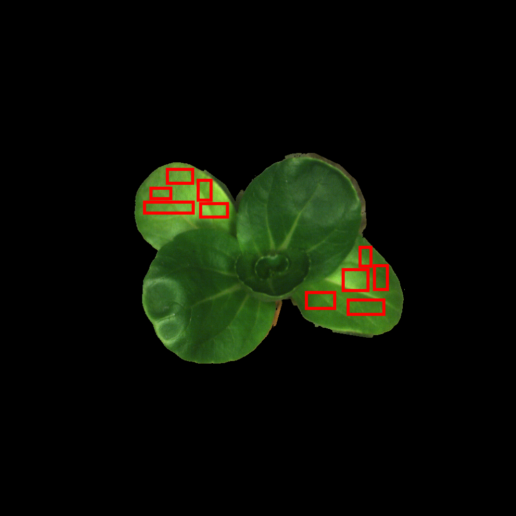
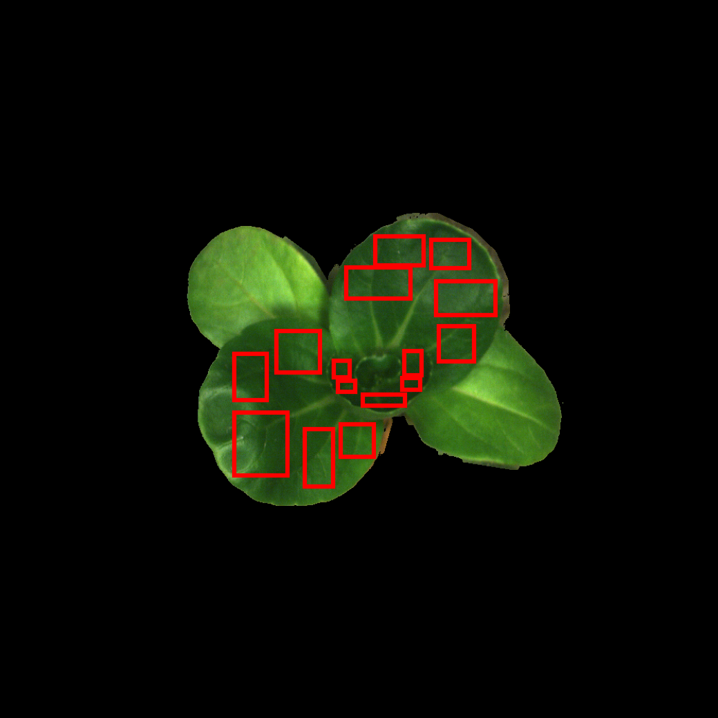
Show raster RGB preview with associated ROIs:
exp.show_image("demo.tiff", "group_1", rgb_band_index=(19, 12, 6), output_path=report_dir + "demo_rast_rgb1.png")
Output:
exp.show_image("demo.tiff", "group_2", rgb_band_index=(19, 12, 6), output_path=report_dir + "demo_rast_rgb2.png")
Output:
2.5. Sample labels and target values
2.5.1 Set sample labels
-
Get current sample label dataframe:
labels = exp.ls_labels()
-
Set new sample labels in the dataframe:
Here we use sample ROI names as sample labels:
labels.iloc[:, 1] = exp.ls_rois_sample(return_dataframe=True, print_result=False)["ROI_name"]
-
Update sample labels:
exp.sample_labels = labels
-
Check sample labels:
exp.ls_labels()["Label"]
Output:
0     1-1
1     1-2
...
24    5-5
2.5.2 Set target values
-
List target value dataframe:
targets = exp.ls_sample_targets()
-
Create mock target values for regression and update target dataframe:
Here we use leaf number:
targets["Target_value"] = [f"leaf_{labl[0]}" for labl in targets['Label']]
-
Load target values from updated target dataframe:
exp.sample_targets_from_df(targets)
-
Check target values:
exp.ls_targets()[["Label", "Target_value"]]
Output:
    Label Target_value
0    1-1       leaf_1
1    1-2       leaf_1
...
24   5-5       leaf_5
3. Design testing pipelines
-
SpecPipe follows a structured data processing workflow with these sequential data levels:
Raster image data -> ROI spectra -> ROI statistics -> Traits to model
-
The data levels in SpecPipe includes:
Raster images: 0 - "image", input image path and output processed image path. 1 - "pixel_spec", if the process callable is applied to 1D spectrum of image pixel 2 - "pixel_specs_array", if the process callable is applied to 2D spectra array of image pixels 3 - "pixel_specs_tensor", if the process callable is applied to 3D spectra tensor of image pixels 4 - "pixel_hyperspecs_tensor", same as "pixel_specs_tensor" but optimized for hyperspectral images ROI spectra: 5 - "image_roi", raster with sample ROIs, for spectrum extraction 6 - "roispecs", 2D array of ROI spectra ROI statistics: 7 - "spec1d", arbitrary 1D data of samples, e.g. 1D spectra, flattened spectra statistical metrics Sample data: 8 - "assembly", sample data list for cross-sample interaction Models: 9 - "model", model evaluation with standard report output as files -
The corresponding data processing workflow is:
Raster image processing:           0 ~ 4
    ↓
Extract ROI spectra:               5 - "image_roi"
    ↓
ROI spectra manipulation:          6 - "roispecs"
    ↓
Summarized ROI spectra:            7 - "spec1d"
    ↓
Sample assembly:                   8 - "assembly"
    ↓
Modeling and model evaluation:     9 - "model"
The processing functions are incorporated in the pipeline according to the specified "data levels". Parallel processes can be added with identical "data level" and "application sequence", and they are arranged using full-factorial approach in the pipeline.
3.1 Create processing pipeline
- Create processing pipeline from SpecExp instance configured above:
from swectral import SpecPipe
pipe = SpecPipe(exp)
3.2 Image processing
-
Create some image processing functions, such as:
-
Standard normal variate:
from swectral.functions import snv
-
Pass-through method for comparison:
def raw(v): return v
3.3 ROI statistics
-
Import spectral statistic metrics for ROI summary:
from swectral import roi_mean, roi_median
3.4 Add models to the pipeline
-
Create some models:
from sklearn.ensemble import RandomForestClassifier
from sklearn.neighbors import KNeighborsClassifier

rf_classifier = RandomForestRegressor(n_estimators=10)
knn_classifier = KNeighborsRegressor(n_neighbors=3)
3.5 Compose and check pipelines
-
Compose pipelines:
pipe.build_pipeline(
    [
        # 1 Image-wide baseline correction
        ((2, 2), [raw, snv]),
        # 2 ROI statistics
        ((5, 7), [roi_mean, roi_median]),
        # 3 Models (Feature selector included)
        ((7, 9), [rf_classifier, knn_classifier], {'validation_method': '2-fold'})
    ]
)
-
Check all processes including models:
pipe.ls_process()
Output:
     Step_0    Step_1         Step_2
0    snv       roi_mean       KNeighborsClassifier
1    snv       roi_mean       RandomForestClassifier
2    snv       roi_median     KNeighborsClassifier
3    snv       roi_median     RandomForestClassifier
4    raw       roi_mean       KNeighborsClassifier
5    raw       roi_mean       RandomForestClassifier
6    raw       roi_median     KNeighborsClassifier
7    raw       roi_median     RandomForestClassifier
4 Execute pipelines
- Run:
pipe.run()
5 Generated reports
-
Pipeline execution data is saved to local storage, use the methods to retrieve reports in the console:
result_summary = pipe.report_summary()
chain_results = pipe.report_chains()
-
Check summary reports
The summary reports include:
result_summary.keys()
Output:
dict_keys([
    'Macro_avg_performance_summary',
    'Marginal_macro_avg_AUC_stats_step_0',
    'Marginal_macro_avg_AUC_stats_step_1',
    'Marginal_macro_avg_AUC_stats_step_2',
    'Marginal_micro_avg_AUC_stats_step_0',
    'Marginal_micro_avg_AUC_stats_step_1',
    'Marginal_micro_avg_AUC_stats_step_2',
    'Micro_avg_performance_summary',
    'sample_targets_stats'])
Demonstration of macro-average performance metrics of classification:
result_summary['Macro_avg_performance_summary']
Output:
    Step_0   Step_1   Step_2  Precision  Recall  F1_Score  Accuracy    AUC
0  2_0_%#1  5_0_%#1  7_0_%#1   0.860000    0.84  0.842828     0.936  0.947
...
7  2_0_%#2  5_0_%#2  7_0_%#2   0.769524    0.72  0.684242     0.888  0.829
Demonstration of marginal macro-average performance metrics of classification:
result_summary['Marginal_macro_avg_AUC_stats_step_0']
Output:
         Process_ID       All   2_0_%#1   2_0_%#2
0     Process_label       All       snv       raw
1         n_records         8         4         4
2    Mean_AUC_macro   0.85425   0.95275   0.75575
3     Min_AUC_macro     0.631     0.942     0.631
4  Median_AUC_macro     0.906    0.9495     0.761
5     Max_AUC_macro      0.97      0.97      0.87
6               All       1.0  0.199557  0.199557
7           2_0_%#1  0.199557       1.0  0.028571
8           2_0_%#2  0.199557  0.028571       1.0
The processes of the step (here raw image and standard normal variates) are compared using non-parametric Mann-Whitney-U test.
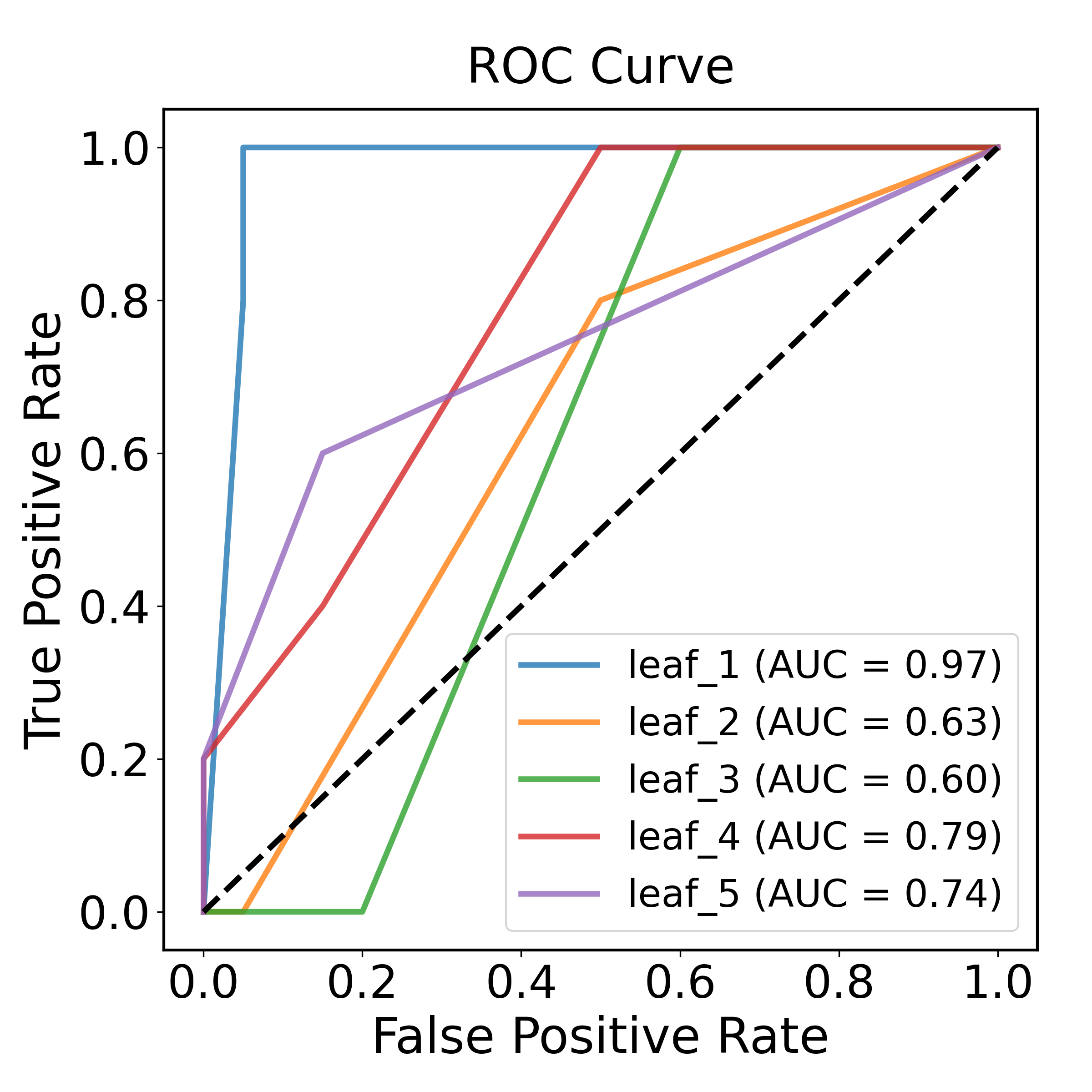
Demonstration of Receiver-Operating-Characteristic curve:
chain_results[0]['ROC_curve']
Output:
6 Regression demonstration
6.1 Create a directory for regression results
-
Create a directory for regression results
report_dir_reg = demo_dir + "/demo_results_regression/"
os.makedirs(report_dir_reg)
6.2 Copy and update the previous pipelines to regression
-
Copy and update SpecExp and SpecPipe instances
import copy

exp_reg = copy.deepcopy(exp)
pipe_reg = copy.deepcopy(pipe)
targets_reg = copy.deepcopy(targets)
-
Update report directory of SpecExp
exp_reg.report_directory = report_dir_reg
-
Modify targets to numeric, here the numbers approaximate the age of the leaves
targets_reg["Target_value"] = [(5 - int(labl[0])) for labl in targets['Label']]
-
Specify the ROIs within a same leaf to a validation group to prevent data leakage
targets_reg["Validation_group"] = [f"leaf_{labl[0]}" for labl in targets['Label']]
-
Update target information using the modified target dataframe
exp_reg.sample_targets_from_df(targets_reg)
-
Check target values and validation groups
exp_reg.ls_targets()[["Label", "Target_value", "Validation_group"]]
6.3 Update the pipeline models to regressors
-
Check and remove classification models
pipe_reg.ls_model()
pipe_reg.rm_model()
-
Update the data manager
pipe_reg.spec_exp = exp_reg
-
Add regressors to the pipeline
Add some regressors:
from sklearn.ensemble import RandomForestRegressor
from sklearn.neighbors import KNeighborsRegressor

rf_regressor = RandomForestRegressor(n_estimators=10)
knn_regressor = KNeighborsRegressor(n_neighbors=3)

pipe_reg.add_model([knn_regressor, rf_regressor], validation_method="2-fold")
6.4 Execute regression pipelines
- Run:
pipe_reg.run()
6.5 Check results of regression pipelines
-
Retrieve reports in console
result_summary_reg = pipe_reg.report_summary()
chain_results_reg = pipe_reg.report_chains()
-
Check summary reports
The summary reports include:
result_summary_reg.keys()
Output:
dict_keys([
    'Marginal_R2_stats_step_0',
    'Marginal_R2_stats_step_1',
    'Marginal_R2_stats_step_2',
    'Performance_summary',
    'sample_targets_stats'])
Demonstration of performance summary content:
result_summary_reg['Performance_summary'].columns
Output:
Index([ 'Step_0', 'Step_1', 'Step_2', 'Mean_Error', 'Standard_Deviation_of_Error', 'Mean_Absolute_Error', 'Normalized_MAE', 'CV_MAE', 'Mean_Squared_Error', 'Root_Mean_Squared_Error', 'Normalized_RMSE', 'CV_RMSE', 'Residual_Prediction_Deviation', 'R2' ], dtype='object') -
Check processing chain reports
For each chain, the reports include:
chain_results_reg[0].keys()
Output:
dict_keys([
    'Chain_processes',
    'Regression_performance',
    'Residual_analysis',
    'Residual_plot',
    'Scatter_plot',
    'Validation_results'])
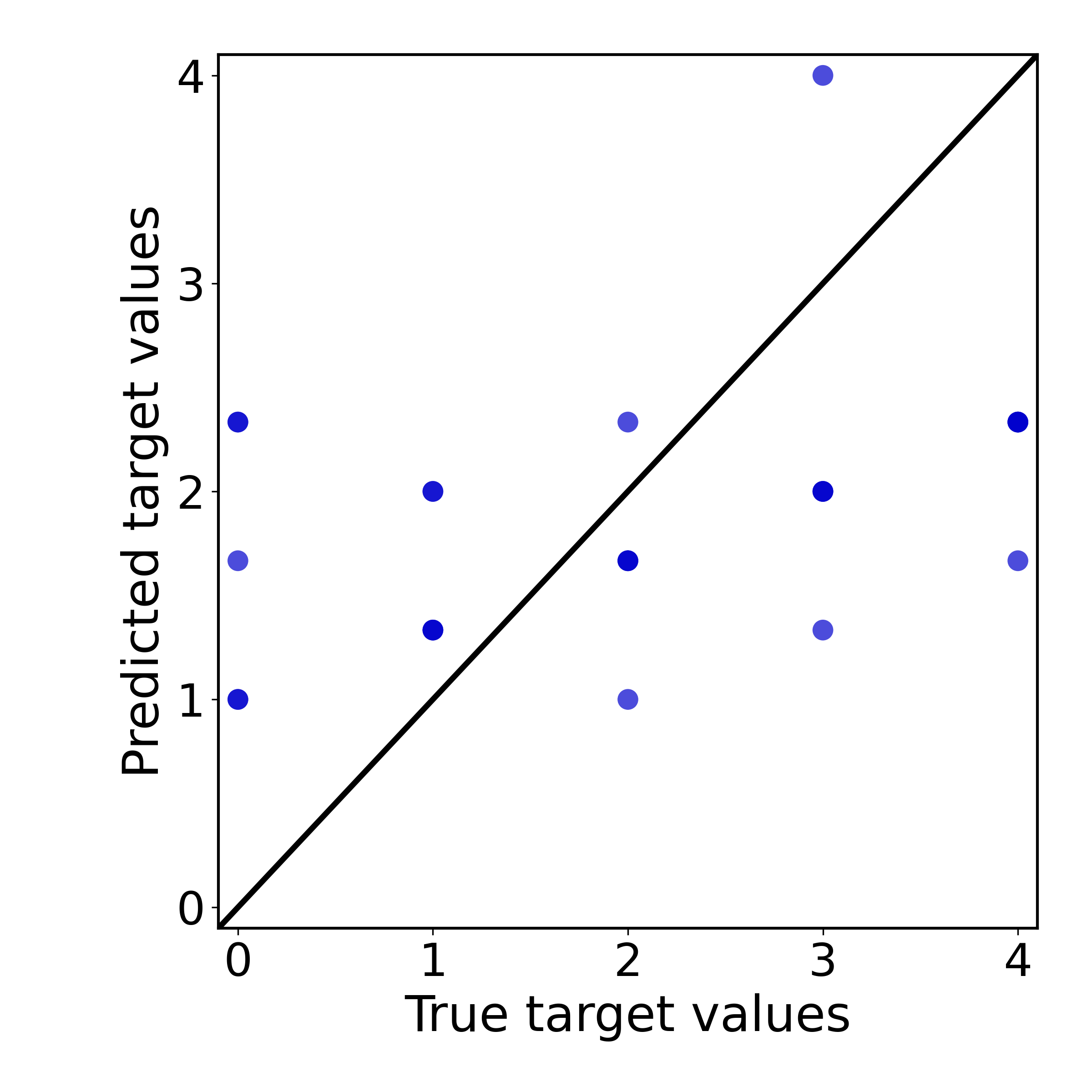
Demonstration of the scatter plot of the processing chain:
chain_results_reg[0]['Scatter_plot']
Output:
7 Feature engineering fittable tests
Feature engineering and resampling fittables (data transformers and resamplers) are fitted during the model validation process and function as integrated parts of the model. To incorporate these transformers, use the model connector functions combine_classifier or combine_regressor (similar to sklearn.pipeline.Pipeline but more flexible and enable swectral pipeline analysis).
-
This module includes a composer that generates batchwise combined models using a full factorial design:
from sklearn.preprocessing import StandardScaler
from sklearn.feature_selection import SelectKBest, f_classif
from swectral import IdentityTransformer  # Passthrough transformer for comparison

selector1 = SelectKBest(f_classif, k=5)  # Select 5 features
selector2 = IdentityTransformer()  # For passthrough (no selection)

from swectral import factorial_model_chains

models = factorial_model_chains(
    [StandardScaler(), IdentityTransformer()],  # Model step 1: test data scalers
    {'Feat5': selector1, 'FeatAll': selector2},  # Model step 2: test feature selection fittables
    # ...
    estimators={'KNN': knn_classifier, 'RF': rf_classifier},  # Estimators (specify custom labels using dictionary input)
    is_regression=False
)
print(models)
Output:
[CombinedClassifier_StandardScaler_Feat5_KNN,
 CombinedClassifier_StandardScaler_Feat5_RF,
 CombinedClassifier_StandardScaler_FeatAll_KNN,
 CombinedClassifier_StandardScaler_FeatAll_RF,
 CombinedClassifier_IdentityTransformer_Feat5_KNN,
 CombinedClassifier_IdentityTransformer_Feat5_RF,
 CombinedClassifier_IdentityTransformer_FeatAll_KNN,
 CombinedClassifier_IdentityTransformer_FeatAll_RF]
-
Add the generated models to your pipeline:
pipe.add_model(models, validation_method="2-fold")
Contributing
Your experience applying this toolset in your specialized field is extremely valuable. Any feedback and contributions are highly welcomed!
- Report bugs: Found an issue? Please open a GitHub issue with details
- Share your domain expertise: Tell us how SpecPipe works (or doesn't work) in your specific application area in discussions
- Suggest features: Have ideas for improvements? Use the GitHub discussions or issues tab
- Submit pull requests: Feel free to fork and submit PRs for bug fixes or small features
- Test and provide feedback: Try it out and let us know about your experience in discussions
License
This project is licensed under the MIT License - see the LICENSE file for details.
Project details
Verified details
These details have been verified by PyPIProject links
GitHub Statistics
Maintainers
Release history Release notifications | RSS feed


Download files
Download the file for your platform. If you're not sure which to choose, learn more about installing packages.
Source Distribution
Built Distribution
Filter files by name, interpreter, ABI, and platform.
If you're not sure about the file name format, learn more about wheel file names.
Copy a direct link to the current filters
File details
Details for the file swectral-0.6.3.tar.gz.
File metadata
- Download URL: swectral-0.6.3.tar.gz
- Upload date:
- Size: 320.3 kB
- Tags: Source
- Uploaded using Trusted Publishing? Yes
- Uploaded via: twine/6.1.0 CPython/3.13.7
File hashes
| Algorithm | Hash digest | |
|---|---|---|
| SHA256 |
30cd33c10fa57c1e78db7efb7335f8d2fd7ffbd469b7b1b1393c903d22ceb899
|
|
| MD5 |
8e5fb99d2a70d888e2d8a84adb62b8b7
|
|
| BLAKE2b-256 |
20286b6817136e0ad5110d1e7e4701effed3ba64609cab6de364b3a97777cfa0
|
Provenance
The following attestation bundles were made for swectral-0.6.3.tar.gz:
Publisher:
build-release.yml on siwei66/swectral
-
Statement:
-
Statement type:
https://in-toto.io/Statement/v1 -
Predicate type:
https://docs.pypi.org/attestations/publish/v1 -
Subject name:
swectral-0.6.3.tar.gz -
Subject digest:
30cd33c10fa57c1e78db7efb7335f8d2fd7ffbd469b7b1b1393c903d22ceb899 - Sigstore transparency entry: 1186315038
- Sigstore integration time:
-
Permalink:
siwei66/swectral@80e0c96ec10643db7b51ed3a67ef517628215e1b -
Branch / Tag:
refs/tags/v0.6.3 - Owner: https://github.com/siwei66
-
Access:
public
-
Token Issuer:
https://token.actions.githubusercontent.com -
Runner Environment:
github-hosted -
Publication workflow:
build-release.yml@80e0c96ec10643db7b51ed3a67ef517628215e1b -
Trigger Event:
release
-
Statement type:
File details
Details for the file swectral-0.6.3-py3-none-any.whl.
File metadata
- Download URL: swectral-0.6.3-py3-none-any.whl
- Upload date:
- Size: 299.2 kB
- Tags: Python 3
- Uploaded using Trusted Publishing? Yes
- Uploaded via: twine/6.1.0 CPython/3.13.7
File hashes
| Algorithm | Hash digest | |
|---|---|---|
| SHA256 |
f6a7a0cdd1ed649343a6929272d6954f6546b7da3733e064619e663966921b1b
|
|
| MD5 |
4d28b64d6be4c2cd43bf86f5e297b80f
|
|
| BLAKE2b-256 |
1ab976fab5edbf74dc85dc8c48e6c0b11c115ee0f610f5d2e1691f6fb9d194c0
|
Provenance
The following attestation bundles were made for swectral-0.6.3-py3-none-any.whl:
Publisher:
build-release.yml on siwei66/swectral
-
Statement:
-
Statement type:
https://in-toto.io/Statement/v1 -
Predicate type:
https://docs.pypi.org/attestations/publish/v1 -
Subject name:
swectral-0.6.3-py3-none-any.whl -
Subject digest:
f6a7a0cdd1ed649343a6929272d6954f6546b7da3733e064619e663966921b1b - Sigstore transparency entry: 1186315040
- Sigstore integration time:
-
Permalink:
siwei66/swectral@80e0c96ec10643db7b51ed3a67ef517628215e1b -
Branch / Tag:
refs/tags/v0.6.3 - Owner: https://github.com/siwei66
-
Access:
public
-
Token Issuer:
https://token.actions.githubusercontent.com -
Runner Environment:
github-hosted -
Publication workflow:
build-release.yml@80e0c96ec10643db7b51ed3a67ef517628215e1b -
Trigger Event:
release
-
Statement type:






