
sympy-editor
A click-to-edit, WYSIWYG-style editor for SymPy
expressions. Expressions are rendered as LaTeX (with KaTeX)
in HTML; every sub-expression is selectable, and a selection can be replaced by
typing new SymPy syntax or by applying SymPy transformations (expand,
factor, simplify, ...). The SymPy expression tree — not the LaTeX — is
always the source of truth.
Works as a Jupyter widget and as standalone HTML (self-contained file, or a local server). Pure Python + plain JavaScript: no node.js, no bundler, no GPL dependencies.
Try it in the browser - a live editor and a shelf of worked derivations, computed on your own machine.
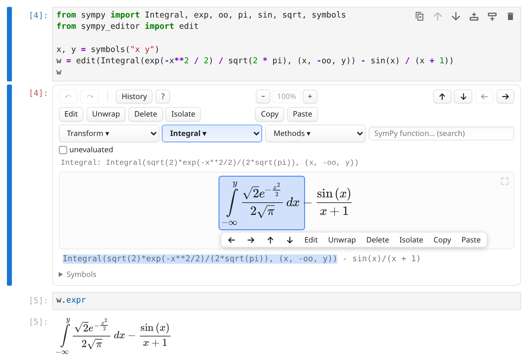
Click any piece of the formula to select it - here the integral inside a larger
expression - then type over it, or apply a SymPy function to that piece alone.
The kernel computes; w.expr is the edited expression, live.
Install
pip install sympy-editor            # core: SymPy only
pip install "sympy-editor[jupyter]" # adds anywidget for the notebook widget
Usage
Jupyter (JupyterLab, Notebook 7, VS Code, Colab...)
from sympy import symbols, sin
from sympy_editor import edit

x, y = symbols("x y")
w = edit(x**2 / y - sin(x))
w            # display the widget and edit in place
w.expr       # the current, edited expression (live)
w.on_change(lambda e: print("now:", e))
The widget runs every edit in the kernel's SymPy (no Pyodide involved).
edit(expr, backend="pyodide") gives instead the self-contained HTML page
that runs its own SymPy in the browser — useful for notebooks exported with
nbconvert, but its edits do not reach the kernel; the default "auto"
picks the kernel widget when anywidget is installed and falls back to Pyodide
with a warning otherwise.
Add-ons in the notebook
Each add-on is a package of its own, so pip install sympy-editor brings
none of them. Install the ones you want — none is on PyPI yet, so from a
checkout — and restart the kernel:
pip install -e addons/sympy_editor_plot -e addons/sympy_editor_latex
pip install -e addons/sympy_editor_tree -e addons/sympy_editor_matching
Every installed add-on is then listed at the top of the drawer the ≡ button opens, to switch on and off while editing, and their Python runs in this kernel — the plot's samples are the kernel's SymPy at work:
from sympy_editor import edit, installed_addons

installed_addons()                               # what this kernel has
edit(sin(x))                                     # every one listed, none on
edit(sin(x), addons=["sympy_editor_plot"])       # on from the start
edit(sin(x), available=["plot", "tree"])         # only these two listed
edit(sin(x), available=[])                       # the editor alone
addons= switches them on, available= says which to list instead of all of
them; each may be named by module, by add-on name, or given as an Addon,
and their front ends are sent when they are switched on, not before. An
add-on whose Python is not installed in the kernel is listed with the reason
rather than silently missing. examples/addons.ipynb walks through it.
on_change is also how the editor drives another widget.
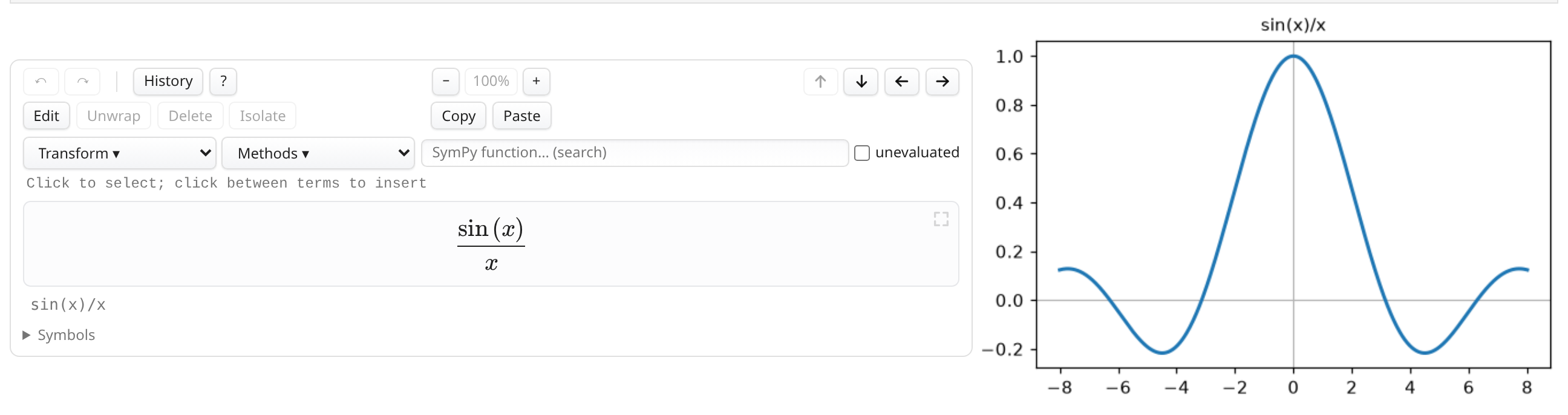
examples/plot_alongside.ipynb puts a graph beside the formula — every
committed edit redraws it, and every free symbol but x grows a slider —
and examples/plot_surface.ipynb does the same to a plotly surface you can
turn around while you edit, updated in place. Both are examples: the wire is
a callback and a traitlet, and the library knows nothing about plotting.
Standalone HTML file
from sympy_editor import save_html
save_html(expr, "expr.html")   # open in any browser
The file is self-contained: it renders immediately and loads
Pyodide + SymPy from a CDN in the background to run
the editing logic inside the browser; a spinner overlay blocks the editor
until they are ready (options={"preload": False} defers that to the first
edit). Use editable=False for a view-only page (still
selectable).
Tutorials: a page that plays itself
A tutorial is the editor page playing a script of timed steps: captions describing what is going on, an arrow and a pulsing ring on whatever is about to be pressed, then the press itself. It is meant to be watched, or recorded as a video. Nothing in the editor's interface starts one, and no ordinary page, server, widget or app carries any of it; only a page built for it plays.
from sympy_editor import save_tutorial_html

save_tutorial_html({
    "expression": "x**2/y - sin(x)",
    "steps": [
        {"at": 0, "caption": "Click any piece of the formula to select it"},
        {"after": 2, "click": {"path": "/1/d"}},
        {"after": 1.5, "click": ".se-toolbar [data-cmd=\"parent\"]", "say": "Up: what holds it"},
        {"after": 1.5, "type": {"target": ".se-source", "text": "(x + 1)**2", "enter": True}},
        {"after": 1.5, "apply": "expand"},
    ],
}, "tutorial.html")
or python -m sympy_editor.tutorial script.json -o tutorial.html. A step
happens "at" a time or "after" the previous one, and never while Python is
still busy with the one before. It does one thing: caption, point, click,
choose, type, key, set, apply, undo/redo, zoom, addons or
wait. A caption goes beside what the step is about, or at the top, centre or
bottom of the editor. When the script is over, everything of the tutorial goes
and the page is the editor as a reader finds it. full_page=False gives a
fragment to embed in a page of one's own; it shares the page's one Python
runtime with any other editor there. sympy_editor/tutorial.py documents every
kind of step.
examples/tutorial/ has a tour of the editor built this way
(python examples/tutorial/build.py). On a page that includes
static/tutorial.js, SympyEditorTutorial.run(editor, script) plays one from
JavaScript.
Local server (scripts, plain Python sessions)
from sympy_editor import serve
new_expr = serve(expr)   # opens the browser; returns when you press "Done"
Editing
| Action | Mouse | Keyboard |
|---|---|---|
| Select sub-expression | click its middle (its left/right edge places a caret before/after it instead; next to a matrix entry or a power's base the caret extends it: + 1 adds, y multiplies) |
↓ (enter children), ←/→ (siblings) |
| Previous / next sibling (or move the caret; with nothing selected, a caret at the start / the end) | ← / → (toolbar and action bar) | ←/→ |
| Select enclosing expression | click again on the same spot, or ↑ | ↑ |
| Go inside: the sub-expression you came up from, or the first one (on an atom: a caret after it) | ↓ (toolbar or action bar) | ↓ |
| Select a range of adjacent terms / factors | drag across them (mouse or pen); on a touch screen hold a finger still on the first one until it is selected, then drag | Shift+→ / Shift+← grow and shrink the range; ←/→/↓ collapse it, ↑ selects the whole sum/product |
| Replace selection by typing | just start typing (SymPy syntax) | |
| Change the operator between two arguments | click the operator itself (+, −, ⋅, =, the − of x − y...): it is selected and a small palette appears; pick + − × ÷ ^ = or Delete (side by side, the two multiply: x + y → xy) |
with the operator selected, type + - * / ^ = < > & |; Del removes it; Esc deselects; ←/→/↓ select an argument, ↑ the node. In a sum * binds just the two terms (x + y + z → xy + z); in a product + splits it there (x·y·z → x + yz). A lone operator typed at a caret does the same |
| Type at a caret | click between two terms, or at the edge of an object: a caret appears; what you type is spliced between its neighbours like in a text editor: operators you type are used as written, a missing one means juxtaposition (cos(t) after x gives x cos(t)), +/- bind at the sum level (x z with +y+ typed between gives x + y + z), , … adds a function argument |
Tab / Shift+Tab put the caret after / before the selection; ←/→ walk it through the formula like a text cursor (into a composite neighbour, out of a node at its ends); ↑ selects the object it is attached to (↓ does nothing at a caret); Enter opens an empty field; Esc removes it |
| LaTeX shortcuts in the field | \theta becomes θ as you type (Greek letters, \infty, \sin, \cdot, \le...); Greek letters are SymPy's names (θ is theta, λ is lamda, ∞ is oo) |
|
| A function at a caret | function box | With a caret shown and nothing selected, the function is added at the caret with an empty box for its argument (sin(□)), the box selected to fill |
| Templates | \int, \sum, \prod, \lim, \diff, \frac, \binom, \matrix |
The whole construction, with faint empty boxes where its parts go: the first box is selected, type to fill it, Tab moves to the next (Shift+Tab back). The boxes are the symbols _1, _2... in the source line |
| A refused edit | The message shows under the formula and the formula flickers red for half a second | |
| Edit selection's existing text | double-click / Edit | Enter |
| Apply / cancel an edit | click elsewhere applies | Enter / Esc |
| Remove the selection entirely (on the whole expression: the formula is emptied and a field takes its place - type the new expression there, it is previewed as you type, Enter applies it; Esc brings the old one back) | Delete | Del |
Remove the node but keep its argument (cos(θ) → θ, ∫f dx → f) |
Unwrap | Backspace — a node with several arguments (x²: the base or the exponent, a sum, a fraction) asks which one to leave, with the one ↑ came from ready to confirm |
Put the node inside a function (x → cos(x), f(x), ∫x dx) |
Document.wrap(path, "cos") / {"action": "wrap"} |
— (the function box calls a function; wrap builds without computing) |
| Keep only the selection (it becomes the whole expression) | Isolate | Ctrl+Shift+I |
| Moving in a matrix or an array | ← → ↑ ↓ | directional, as it is drawn: along the row, between the rows, for the selection and the caret alike (an array of any rank too - a rank-3 one is a row of matrices, and → crosses into the next block). At the edge the usual meaning takes over: ↑ in the top row selects the matrix itself |
| Rows and columns of a matrix | in a matrix (the matrix, or anything in an entry) the action bar has + row / + col (a new row / column of empty slots after the selected one; after the last for the matrix itself) and − row / − col (the selected one removed); the grip at the matrix's bottom-right corner reshapes it when dragged - the same entries laid out another way, so it snaps to the shapes that hold them all (12 entries: 1×12, 2×6, 3×4, 4×3, 6×2, 12×1), nothing added or lost | Document.insert_row/insert_col/delete_row/delete_col(path), reshape_matrix(path, rows, cols), resize_matrix(...) (grows and truncates), {"action": "matrix", "op", "rows", "cols"} |
| Transform the selection | pick an operation in the Transform ▾ menu (general) or the type menu ("Matrix ▾", "Array ▾"...) - the first group of the last toolbar row, both lists chosen by options={"actions": ...}: it applies at once, or asks for what it needs first (the array tools want their axes) |
|
| Matrix ↔ array | "Matrix ▾ → As array"; "Array ▾ → As matrix (rank 2)" — a MatrixSymbol becomes an ArraySymbol (entries stay implicit), an explicit matrix an explicit array |
|
| Array tools | "Array ▾" (for explicit arrays and array symbols): permute axes (1, 0), contract axes (0, 1), diagonal over axes, reshape, rank, explicit entries |
|
| Reshape | "Matrix ▾" / "Array ▾" → Reshape… — a matrix reshaped to a rank other than 2 becomes an array | |
| Derive by array | Transform ▾ → Derive by array… — by x or [x, y], for an expression (its gradient), a matrix or an array, symbolic or explicit |
|
| Copy / cut / paste a part | Copy / Paste (toolbar or action bar) | Ctrl+C / Ctrl+X copy the selection's SymPy source; Ctrl+V pastes over a selection or at a caret |
| Apply any SymPy function | the function box in the toolbar (the library group, beside Methods): it lists every function of SymPy, type to narrow the list, pick one; a function that needs parameters asks for them (symbol parameters offer the selection's free symbols — solve on sin(x)cos(y) asks x or y); diff(x), .T, det() typed in full apply as written |
|
| Call a method of the selection's class | the Methods menu (the library group) lists every public method and property of the selected object's class (of the whole expression when nothing is selected) — .det(), .T, .rref() on a matrix, .diff(), .as_poly() on an expression; picking one calls it, and a method that needs parameters asks for them. A Lambda is itself a function: its menu starts with ( ) apply, which asks for the arguments and evaluates it there ((3) in the function box does the same) |
|
| Undo / redo | ↺ / ↻ | Ctrl+Z / Ctrl+Shift+Z |
| Zoom the formula | − / 100% (reset) / +, Ctrl+mouse wheel, pinch with two fingers | Ctrl+plus / Ctrl+minus / Ctrl+0 |
| Scroll a formula wider (or, in full screen, taller) than the view | the arrow strips along the edges it runs past (each scrolls a screen and goes once that end is in sight), the scrollbar, the mouse wheel over the formula, a drag on its empty space; on a phone one finger dragged anywhere across it, or two fingers moving together |
A small action bar appears under whatever is selected — ↑ parent, ↓ inside, Edit, Unwrap, Delete, Copy — so these actions are one click or one tap away from the object; the same commands sit in the toolbar and on the keys.
Editing happens inside the formula: the selected node is swapped for a small
text field at its position, and the formula re-renders when you press Enter.
A selection and an insertion caret never coexist: with a selection, typing
replaces it; with a caret, typing only inserts. A range (b + c inside a + b + c + d) is
edited, deleted and transformed like a single node: typing replaces it, Del
removes its terms, an operation picked in a menu transforms just those terms.
On phones and tablets: tap to select, tap the selected node again to edit it, tap a gap for a caret and tap it again to insert, tap an operator to change it from its palette; hold a finger still on a node until it is selected, then drag across its neighbours to select a range - dragging to the edge of the view scrolls the formula along and keeps taking in what appears, so the range reaches terms that were off the screen; the toolbar has ↑ for the parent and a keyboard button that opens the keyboard for the selection, the caret or the whole expression; the menus apply an operation as soon as it is picked. Two fingers zoom the formula and, when it is larger than the view, scroll it; one finger dragged across it scrolls it sideways (a plain swipe never selects, so a tap that wobbles is still a tap); the arrow strips at the edges scroll a screen at a time; and vertical swipes still scroll the page. Transformations act on the selected sub-expression only (on the whole formula when nothing is selected).
Typed input is parsed with sympy.parsing.sympy_parser.parse_expr in the
context of the expression, so existing symbols keep their assumptions and
undefined functions (and MatrixSymbols / IndexedBases) are reused. Names
that do not occur in the current expression become plain symbols - unless the
node being replaced is a matrix, in which case they become MatrixSymbols of
its shape (so C.T typed over B in A*B works). Ancestors are rebuilt
with SymPy's normal automatic evaluation (replacing y by -x in x + y
gives 0). LaTeX is not typed input: the
LaTeX add-on reads it, with its
ambiguities laid open (see Add-ons).
Names vs. SymPy functions. A typed name is resolved in this order: a
symbol declared in the Symbols panel (or passed as symbols=), a name already
in the expression, then SymPy's own names (sin, pi, E, I, gamma,
...), and finally a new plain symbol. So a variable called sin is declared
once in the panel and wins from then on; for a one-off, write it in backticks
(`sin`*x); \sin is always the function. When a name you typed was
taken as SymPy's function or constant, the status line says so and points at
these two options.
What you select and edit is what you see, even where SymPy's tree differs
from the rendering: the 1 of 1/n (the tree holds Pow(n, -1)) is a node
of its own and typing x there gives x/n; in 1/(2e) (the tree's
exp(-1)/2) the 2 and the e of the denominator are editable, and so is
the denominator 2e as a whole; a denominator raised to a power ((x+1)**2
in x/(x+1)**2, the tree's Pow(x + 1, -2)) is edited as shown, exponent
included; in x - 2y the 2 is the 2 you see.
The Symbols panel under the formula lists every name with what it stands
for (Symbol with its assumptions, MatrixSymbol with its shape, Function,
...) and lets you change it throughout the expression: make y a 2×2
MatrixSymbol, an explicit Matrix of y[i, j] entries (symbolic dimensions
such as n are fine for a MatrixSymbol), or a positive real Symbol
(assumptions are a comma-separated list). Products and powers are rebuilt as
MatMul/MatPow; a change SymPy cannot represent (a matrix under a
transpose back to a scalar) is refused with its error. The last row of the
panel declares a new name before you type it — so C typed into a
scalar context can still be a 3×3 matrix symbol — and from Python the same is
edit(expr, symbols=[MatrixSymbol("C", 3, 3)]) or
w.document.declare("C", "MatrixSymbol", 3, 3).
The last row of the toolbar holds what can be applied, in two groups boxed apart. The four menus in them are one kind of control: a box that lists everything it offers when it takes the focus, narrows the list as you type, and picks with ↑/↓ + Enter or a click.
The first group is the actions. The Transform ▾ menu holds the
general ops (simplify, expand, factor, ...) and applies one as soon as it is
picked. Operations specific to the selection's type appear in the
type menu next to it, labelled with the type
("Matrix ▾", "Integral ▾", "Equation ▾"...), and apply as soon as you pick
one: transpose / inverse / trace / determinant / as_explicit for matrices,
evaluate / numeric value / expand or simplify the function inside for
integrals, sums, derivatives and limits, swap sides / move everything to the
left / simplify or expand both sides for equations, tomatrix for arrays.
Both lists are yours to choose: options={"actions": {...}} names, per
menu, the ops to offer and their order - "expr" for Transform, a kind
("matrix", "integral", "relational"...) for the type menu of
selections of that kind; an entry is an op's name, or {"name": ..., "label": ...} to relabel it; a key left out keeps every registered op:
edit(expr, options={"actions": {
    "expr": ["simplify", "expand", {"name": "factor", "label": "Factorise"}],
    "matrix": ["transpose", "determinant", "inverse"],
}})
The second group is the library, which is never trimmed: the Methods ▾ menu lists every public method and property of the selected object's class, and the function box every function of SymPy.
Matrices (dense and sparse), MatrixSymbol expressions, block matrices,
determinants/traces and N-dimensional Arrays are supported: every entry is
selectable and editable, and the container is rebuilt around the edit (see
examples/demo_matrices.py and examples/demo_matrices.ipynb). An explicit
matrix also changes shape in place: with the matrix or one of its entries
selected, the action bar adds and removes rows and columns (new entries are
empty slots to fill, like a template's), and the grip at its bottom-right
corner reshapes it by dragging: the same entries laid out another way, as
Matrix.reshape does, snapping to the shapes that hold every one of them.
Register your own transformations, for every selection or only for some
kinds ("matrix", "array", "scalar"; the mapping from kinds to SymPy
types is sympy_editor.ops.KINDS):
from sympy_editor import register_op

@register_op("my_op", label="My op")
def my_op(expr):
    return ...

@register_op("gram", label="Gram matrix", kinds=("matrix",))
def gram(m):
    return m.T * m
Mobile apps
mobile/ packages the same editor page as a minimal Android (Kotlin WebView)
and iOS (SwiftUI WKWebView) app: python mobile/build_www.py produces the
shared, offline-capable bundle, and each platform folder is a few files that
just display it.
Both apps run Python themselves: CPython and SymPy are packaged in the app
- Android through Chaquopy, iOS through
Python.xcframework- and the page edits through the app's own interpreter (thenativebackend), so there is no WebAssembly runtime to start and no Pyodide in the bundle - faster to open, and the same SymPy as on the desktop. Android 7.0 (API 24) and iOS 15. Only the web app still runs Python in the page, with Pyodide. Seemobile/README.md.
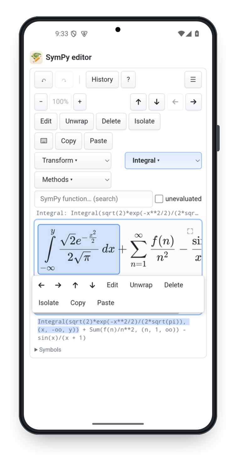
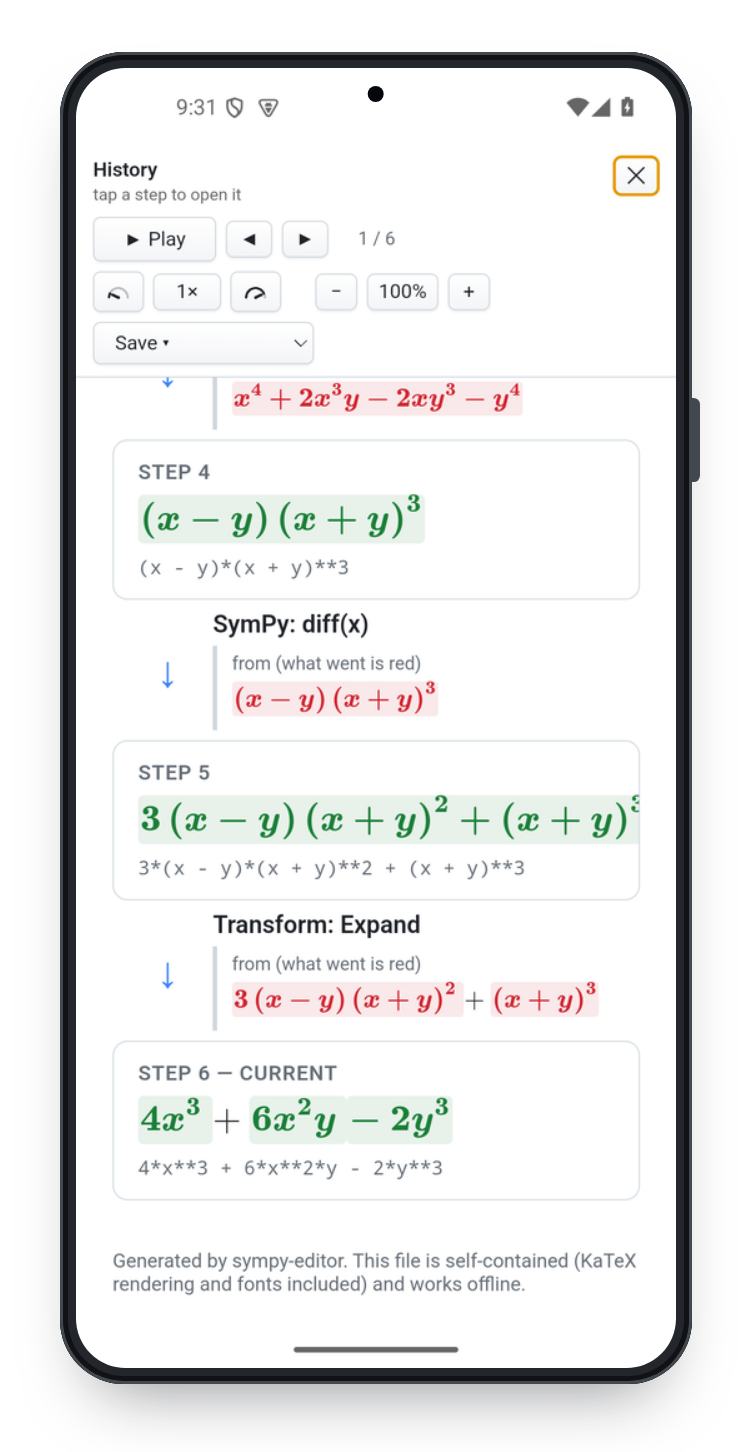
The same editor on a phone, and the history of a session read back step by step - what each step changed in red and green. Both computed on the device, offline. They are also on the live page, in context: screenshots of the apps.
Mac app
python desktop/build.py --run builds the editor as a Mac application and
opens it: the same page in a window, editing in the app's own CPython.
Nothing is installed and nothing is downloaded at run time - the interpreter,
SymPy and the add-ons are inside the .app (about 180 MB), which runs on
macOS 11 and later, on Apple silicon and Intel alike.
It is the iOS app's shell in a window - the same Swift and Objective-C, with a
few #if os(macOS) branches - so a fix to one is a fix to both. The
interpreter is the macOS build of the release the iOS app pins, which carries
the standard library inside Python.framework, so the app embeds the
framework and installs nothing. To hand the app to someone else, sign it with
a Developer ID certificate and notarize it; see desktop/README.md.
Web app
python webapp/build.py builds the same page as an installable, offline-capable
web app (a PWA) in webapp/dist/: the bundle plus a manifest, icons and a
service worker that caches everything on the first visit. Sessions, history
and zoom live in the browser's storage, as in the app. --serve tries it at
http://127.0.0.1:8000/; dist/ is a static site for any https host, and
.github/workflows/webapp.yml publishes it with GitHub Pages (enable Pages
with "GitHub Actions" as the source once).
The source line
The SymPy source under the formula and the formula itself are one document seen twice, and the two follow each other both ways. Select a piece of the text and the corresponding sub-expression is selected in the formula; select in the formula and the matching source text is highlighted, a negated term with its sign. Put the text cursor in the line and a caret appears at the same place in the formula (whatever was selected is dropped, as it would be in a text editor); move the caret in the formula and a cursor shows where it stands in the text. The line is editable and previews as you type: whenever the text parses, the formula above shows it (a text that does not parse marks the line red and leaves the formula alone); Enter commits it — as one undo step — and Esc reverts. That is where whole-expression edits happen: the rendered formula itself is never replaced by code.
What changed
A committed change is animated: the parts of the old formula that disappear
turn red and slide towards their replacements while fading out, the new
parts fade in in green (and stay green until you touch the formula
again), and the parts that survive slide to their new places
(options={"animate": False} turns it off; it is off under
prefers-reduced-motion). What changed also keeps a very faint tinted box
behind it - one box per changed sub-expression, covering it whole, however
tall it is (a fraction, a matrix with its brackets).
Evaluated or unevaluated
The unevaluated toggle next to the function box decides what a
transformation or a SymPy function produces: off, the result is computed
(the determinant of a numeric matrix is a number); on, its symbolic form is
built - Determinant(M), Inverse(A), Transpose, Trace, Derivative(f, x) for diff(x), Integral(f, x) for integrate(x), Limit, Sum,
Product, Subs, and sin(0), sqrt(4), exp(0)... left as written - to
be evaluated later with Evaluate (doit). A transformation that has no
such form (Simplify, Expand, Factor...) is applied as usual and the status
line says so. The history records the choice ("Transform: Determinant
(unevaluated)").
History view, report and script
History (toolbar, or View… in the drawer's History) shows the current history in the page: every step rendered, what a step brought in green, and between two steps an arrow with what produced the change (a transformation from the menu, a SymPy function, an edit, typed text...) and the previous formula with what went in red. Bold colour and a faint box mark exactly what the step touched, nothing around it. Tapping a step opens it in the editor. From there:
- Play runs the history as a slideshow: one slide per step, with the change that produced it - what it was in red, what it became in green - on the same screen, large and centred, advancing on its own.
- ◀ ▶ step through the slideshow while it is paused, and walk the whole history when it is not playing at all: each press scrolls to the next step and marks it, and Play carries on from there.
- − / + in the same strip set the size of the formulas, in the listing and in the slideshow alike; Ctrl+wheel and two fingers do the same. On a page of its own the whole panel can be dragged taller or shorter. Its controls sit in the strip above, which stays put while the steps go by; inside the report the same keys work (space pauses, ← → step, Esc shows the whole history again). The player travels with the page, so a saved report plays on its own too.
- Save ▾ offers the two ways out. As a web page downloads the same view as a self-contained HTML file: KaTeX's rendering and fonts are inlined, so it works offline and can be shared as it is.
- As a Python script downloads a script that rebuilds every step with SymPy
alone (
from sympy import *, the declarations of the names used - assumptions, matrix shapes, functions -, then oneexpr = ...per step with what produced it as a comment, all collected insteps); run it or import it.
Browsers download the files (or offer the share sheet where the Web Share API takes files); the Android app saves them in Downloads and opens the share sheet.
The history viewer on its own (no editor)
The step-by-step view is not part of the editor: it needs a list of expressions and a word about what turned each into the next, whoever computed them. So a derivation carried out in Python - the steps of an integration, a chain of rewrites, the output of somebody else's algorithm - is shown exactly the way the editor shows its own sessions, with the same diffs:
from sympy import Integral, cos, sin, symbols
from sympy_editor import History, save_history_html

x = symbols("x")
steps = History([
    Integral(x * sin(x), x),
    (-x * cos(x) + Integral(cos(x), x), "by parts: u = x, dv = sin(x) dx"),
    (-x * cos(x) + sin(x), "the remaining integral"),
], title="∫ x sin(x) dx, by parts")

save_history_html(steps, "steps.html")      # a page of its own
History(steps, ...)takes expressions or(expr, "what produced it")pairs;History.add(expr, action)appends one at a time, so a loop can build the history as it computes;History.from_document(doc)takes an editing session's own.to_history_html(steps, full_page=False)gives an embeddable fragment anddisplay_history(steps)shows it in a notebook cell (no kernel round trip: the page is static).- Both accept a
History, aDocument, or just a list of expressions.
The page runs no Python: it renders the steps with KaTeX in the browser, and
its Save as web page button writes the whole thing - fonts included - to
one offline file. examples/demo_history.py builds one.
python webapp/build.py --shelf DIR writes that shelf as a page that
introduces the project with every derivation embedded in it, an editor
beside it and KaTeX with them: about 1.5 MB, a folder to drop into any site.
That page is what https://upabjojr.github.io/sympy-editor/ serves. The full
web app build puts the same page at dist/derivations/.
examples/derivations/ is a shelf of worked derivations built this way -
the quadratic formula by completing the square, the Gaussian integral, the
geometric series, Euler's identity, a derivative from first principles,
partial fractions, the eigenvalues of a matrix, Gaussian elimination, the
harmonic oscillator from its Lagrangian, least squares. python examples/derivations/build.py --open writes a page for each and an index
over them.
examples/manualintegrate_steps.ipynb shows the point of the separation: it
flattens the rule tree that sympy.integrals.manualintegrate.integral_steps
returns into a list of expressions - one rule per step, by parts, by
substitution, term by term - and hands it to the viewer, so SymPy's own
reasoning can be read (and played) like any other derivation. That code
lives in the notebook: the library knows nothing about manualintegrate.
Long computations
A transformation that takes a while does not freeze the page: after a moment
a spinner overlay names what is being computed, and after a couple of seconds
it offers an Interrupt button, which stops the computation and leaves the
expression as it was. In standalone pages Python runs in a Web Worker and is
restarted on interruption (the undo history of the page is lost then; a
file:// page in Chromium cannot create the worker and runs Python in the
page instead, without interruption); the local server and the Jupyter widget
interrupt the thread doing the work (interrupt_thread), so nothing else is
lost.
Sessions and history (mobile app, or options={"sessions": True})
The ≡ button opens a lateral drawer, out of the widget, listing your
sessions — expressions, each with its own undo history, kept in the
browser's storage. New session… offers an empty formula (the default:
you type it in the source line), a copy of the current expression, or one
of the built-in examples (sympy_editor.examples); Open switches (the
one you leave is saved first); Delete (click twice) removes one. The
current session is a card, and its History is a sub-tab inside that
card: one row per step, each shown as a diff - the previous formula with
what went in red, then this one with what came in green - and clicking a
row goes back (or forward) to that step. Tapping a session's row opens
it. Available on Pyodide-backed pages.
The formula sits on its own faintly outlined canvas, with the SymPy source of the whole expression under it and the tools above. A quasi-transparent button in the canvas's top-right corner gives the formula the whole screen: the editor covers the page, everything else - the tools, the source line, the Symbols panel - steps aside, and the formula alone is drawn large in the middle. It is real full screen where the platform has one - the browser's own (the Fullscreen API), and in the Android app the status and navigation bars go too. The same button - or Esc, when nothing is selected - comes back.
The toolbar's ? opens this whole guide inside the editor - every gesture, key and tool in one box (Esc closes it).
The toolbar is organised in three rows of related blocks: the session and its timeline (sessions, undo/redo, History, ?, Done) with the zoom; the selection (navigation arrows, then Edit/Unwrap/Delete/Isolate and the clipboard); and what to apply (the Transform, type and Methods menus, the function box, the unevaluated toggle). The blocks sit in columns - three from 44rem, and on a narrow screen they spread across each line instead - so the left column starts at the left edge, the right one ends at the right edge, and the strip reads as a grid rather than a wall of buttons. A block never breaks apart: what belongs together stays together, and the action bar under a selection wraps the same way, so every button stays reachable.
Add-ons
The editor can be extended from outside: an add-on is a package of its own
that gives a document node types from another library, transformations,
data beside every snapshot and methods of its own, and a panel of HTML and
JavaScript under the formula - through one contract,
sympy_editor.addons.Addon, and one message. Four drafts live in
addons/: the expression tree as an editable graph,
the graph of the selection drawn by Plotly.js, rewrite rules with
wildcards matched many-to-one by
sympy-matching, and LaTeX
import - a box under the formula that reads LaTeX with an Earley parser
(through Lark), offers a menu for
every ambiguous part (f(x) applied or multiplied, how far \sin x \cos y
reaches) and a switch for every constant name (\pi the constant, or a
symbol called pi), and puts the reading over the selection or in place of
the whole expression.
An add-on is a package of its own, made by anyone, found by the editor
once it is installed (pip install -e addons/sympy_editor_tree for a
draft; a published one with plain pip install). Then every way of
starting the editor takes addons=:
from sympy_editor import edit, save_html, serve, installed_addons
installed_addons()                                       # {'matching': ..., 'plot': ..., 'tree': ...}
w = edit(sin(x)**2 / x, addons=["tree", "plot", "matching"])          # Jupyter, by name
save_html(expr, "page.html", addons=["tree", "plot"])                  # a self-contained page
serve(expr, addons=["matching"])                                       # the local server
The Add-ons section at the top of the ≡ drawer switches any installed add-on on or off
while editing. Not installed? A module name (addons=["sympy_editor_tree"])
or the object itself (addons=[ADDON]) work too; python addons/demo.py
builds a page with the four drafts straight from the checkout.
addons/README.md describes the architecture, and addons/template/ is
an add-on to copy when writing your own.
How it works
sympy_editor.AnnotatedLatexPrinter extends SymPy's LatexPrinter so that
every printed sub-expression is wrapped in KaTeX's \htmlData{path=/1/0}{...}
(AnnotatedStrPrinter does the same for str(), and latex_spans(expr) /
annotate_str(expr) give the character spans of every node in both strings,
keyed by the same paths).
KaTeX turns that into <span data-path="/1/0">, so the DOM knows which node
of the expression tree each glyph belongs to. Editing operations
(Document.replace/delete/insert/operator/apply/call/undo/redo) rebuild the
tree and re-render.
See AGENTS.md for the architecture and design notes, and
docs/cursor-and-selection.md for what the
cursor and the selection do - the one description the page, the server, the
Jupyter widget and the apps all follow.
Dependencies and licences
| Component | Licence | How it is used |
|---|---|---|
| SymPy | BSD-3 | required |
| anywidget (+ ipywidgets, traitlets) | MIT / BSD-3 | optional, Jupyter widget |
| KaTeX | MIT | loaded from a CDN by the browser (URL configurable) |
| Pyodide | MPL-2.0 | loaded from a CDN by the browser, standalone HTML only |
| SymPy wheel (PyPI) | BSD-3 | loaded by the browser into Pyodide (the newest SymPy, ahead of Pyodide's own package) |
sympy-editor itself is BSD-3-Clause.
Development
pip install -e ".[jupyter,test]"
pytest                           # Python tests (printer, document, HTML, server, widget)
python examples/demo.py          # writes examples/demo.html (regenerate after code changes:
python examples/demo_matrices.py #  the pages embed the package; tests/test_examples.py checks they are current)
python examples/demo.py --serve  # local-server mode
jupyter lab examples/demo.ipynb  # notebook demo (plot_alongside.ipynb plots what you edit)
Browser end-to-end tests of the JavaScript front end use Playwright (dev-only, Apache-2.0, never shipped) and a real headless Chromium:
pip install playwright && python -m playwright install chromium
pytest tests/test_browser.py                       # needs network for the KaTeX CDN
SYMPY_EDITOR_SLOW_TESTS=1 pytest tests/test_browser.py   # also the Pyodide page
They are skipped automatically when Playwright, the browser or the network
are unavailable. Graphical edits are tested as user scenarios with the
Scenario helper in tests/test_browser.py (scenario(expr).caret_after(path) .type("+ B*A").enter() then .source), run on both the HTTP backend and a
Pyodide page. .github/workflows/ci.yml runs everything on push.
1 maintainer

Download files
Download the file for your platform. If you're not sure which to choose, learn more about installing packages.
Source Distribution
Built Distribution
Filter files by name, interpreter, ABI, and platform.
If you're not sure about the file name format, learn more about wheel file names.
Copy a direct link to the current filters
File details
Details for the file sympy_editor-0.1.1.tar.gz.
File metadata
- Download URL: sympy_editor-0.1.1.tar.gz
- Upload date:
- Size: 366.1 kB
- Tags: Source
- Uploaded using Trusted Publishing? No
- Uploaded via:
twine/7.0.0 CPython/3.12.3
File hashes
| Algorithm | Hash digest | |
|---|---|---|
| SHA256 |
22783acb161907a76b08a94750fbe9f9bdb642651820d6b820e1a573d52b7ad3
|
|
| MD5 |
9789388f1777474c31a852b9567d3170
|
|
| BLAKE2b-256 |
00c79dc367e28e37dd3aebfb8d06e5bd57034dcf78534344c9b6e29d84cd3c2f
|
File details
Details for the file sympy_editor-0.1.1-py3-none-any.whl.
File metadata
- Download URL: sympy_editor-0.1.1-py3-none-any.whl
- Upload date:
- Size: 216.3 kB
- Tags: Python 3
- Uploaded using Trusted Publishing? No
- Uploaded via:
twine/7.0.0 CPython/3.12.3
File hashes
| Algorithm | Hash digest | |
|---|---|---|
| SHA256 |
8521e57eab434a40e4e997014df63516fd6cf6803a47f334e31730882d5522d2
|
|
| MD5 |
b57a3157f5872eb938a9be6bc799c0ac
|
|
| BLAKE2b-256 |
6f75f40f43097e37f46d573ecd7389ba35385398dba3cc0fc8543aba77cb1f4f
|














