
🔬 TanabeSugano
A Python-based Eigensolver for Tanabe-Sugano & Energy-Correlation Diagrams
Interactive visualization of d-orbital splitting in transition metal complexes
📊 Build & Quality



📦 Package Info




📚 Resources



🚀 Quick Start • ✨ Features • 📖 Documentation • 🎨 Examples • 🤝 Contributing
📋 Table of Contents
- Overview
- Upgrading to 2.0.0
- Quick Start
- Features
- Usage
- Examples
- Interactive Diagrams
- Scientific Background
- Contributing
- Citation
- License
🌟 Overview
TanabeSugano is a comprehensive Python package for calculating and visualizing Tanabe-Sugano and Energy-Correlation diagrams for d2-d8 transition metal ions. Based on the pioneering work of Yukito Tanabe and Satoru Sugano, this tool provides both computational accuracy and interactive visualization capabilities.
Why TanabeSugano?
- 🎯 Accurate Calculations - Based on rigorous quantum mechanical principles
- 📊 Beautiful Visualizations - Generate publication-quality diagrams
- 🔄 Interactive Exploration - Explore diagrams with Plotly integration
- 🚀 Easy to Use - Simple CLI and Python API
- 📱 Cloud-Ready - Run in Google Colab or locally
🔄 Upgrading to 2.0.0
2.0.0 is a breaking release. Three changes bite existing users; the full list is in
CHANGELOG.md.
| What changed | Migration |
|---|---|
matrices.dN.solver() returns a LevelSet, not dict[TermKey, Float64Array]. LevelSet is not a Mapping — states[key], .items() and len() raise TypeError. |
Call .as_dict() for the old shape, or iterate .levels. A bare dict could not express a multiplet: for d⁸ it mapped 3_T_1 to a two-element array, so ν₂ and ν₃ were indistinguishable. |
Term keys renamed: 1_T_3 → 1_T_2 (no T₃ irrep exists in Oh) and *_E_1 → *_E (Eg carries no subscript). |
Update any literal key match. TermKey now makes both old spellings unwritable. This also renames the corresponding CSV columns in ts-diagrams/**. |
Committed CSV artifacts changed. delta_B held Dq/B while labelled Δ/B and is now 10× larger (the old values were wrong); the cm⁻¹→eV factor was 0.00012 and is now 1/8065.54; columns are renamed as above and now sorted rather than dict-insertion ordered. |
Re-read any pinned column indices by name. Values are otherwise unchanged — verified cell-by-cell across all 42 regenerated files, and now guarded by a --check step in CI. |
Python ≥ 3.12 is required.
🚀 Quick Start
Installation
Choose your preferred installation method:
# 📦 Install from PyPI (recommended)
pip install TanabeSugano

# 🔧 Install with interactive plotting support
pip install TanabeSugano[plotly]

# 🤖 Install with MCP server support (Claude Desktop, Cursor, VS Code, …)
pip install TanabeSugano[mcp]

# 🌐 Install from GitHub (latest development version)
pip install git+https://github.com/Anselmoo/TanabeSugano.git
Note: TanabeSugano now uses the
uv_buildbackend and requires Python ≥ 3.12.
Basic Usage
Generate a Tanabe-Sugano diagram in seconds:
# Generate diagram for d6 configuration
tanabesugano -d 6

# Customize parameters
tanabesugano -d 6 -Dq 8000 -B 860 1.0 -C 3850 1.0
🎮 Try it now:
✨ Features
📖 Usage
Command Line Interface
🔧 View all CLI options
$ tanabesugano --help
usage: tanabesugano [-h] [-d D] [-Dq DQ] [-cut CUT] [-B B B] [-C C C] [-n N] [-ndisp]
                    [-ntxt] [-slater] [-v] [-html] [-html-offline]

A python-based Eigensolver for Tanabe-Sugano- & Energy-Correlation-Diagrams based on
studies by *Yukito Tanabe and Satoru Sugano* for d3-d8 transition metal ions: For
further help, please use tanabe '--help'

options:
  -h, --help     show this help message and exit
  -d D           Number of d electrons, 2-8 (default d5)
  -Dq DQ         10Dq crystal field splitting (default 10Dq = 8065 cm-)
  -cut CUT       10Dq crystal field splitting (default 10Dq = 8065 cm-)
  -B B B         Racah Parameter B and the corresponding reduction (default B = 860 cm-
                 * 1.)
  -C C C         Racah Parameter C and the corresponding reduction (default C =
                 4.477*860 cm- * 1.)
  -n N           Number of roots (default nroots = 500)
  -ndisp         Plot TS-diagram (default = on)
  -ntxt          Save TS-diagram and dd energies (default = on)
  -slater        Using Slater-Condon F2,F4 parameter instead Racah-Parameter B,C
                 (default = off)
  -v, --version  Print version number and exit
  -html          Save the interactive Plotly diagrams as HTML (default = off)
  -html-offline  With -html, write a shared plotly.min.js beside the diagrams so they
                 render without a network connection (default = CDN)
The MCP layer uses per-configuration Racah defaults rather than the CLI's single d5 free-ion pair — see
src/tanabesugano/mcp/_defaults.py.
Python API
Changed in 2.0.0.
solver()returns aLevelSet, not adict.LevelSetis not a Mapping —states[key],.items()andlen()raiseTypeError. Call.as_dict()for the previous shape, or iterate.levels.
from tanabesugano.levels import LevelSet

# Solve the d8 manifold at one ligand-field strength.
manifold = LevelSet.solve(8, dq=850.0, b=1030.0, c=4850.0)

print(manifold.ground.label)          # 3_A_2
print(manifold.level_count)           # 11 levels ...
print(manifold.total_degeneracy)      # ... accounting for C(10,8) = 45 microstates

# Levels are typed objects, not bare arrays, and carry free-ion parentage:
# 3T_1g(F) / 3T_1g(P), the notation the literature uses, rather than a
# positional (a)/(b).
for level in manifold.spin_allowed():
    print(f"{level.parent_unicode:10} {level.energy_cm1:9.1f} cm-1")
# 3T_2g        8500.0 cm-1     <- nu1 = 10Dq exactly, for d3 and d8
# 3T_1g(F)    14283.0 cm-1
# 3T_1g(P)    26667.0 cm-1

# Name a transition the way a caption would.
excited = manifold.for_term("3_T_1")[1]
print(manifold.transition_unicode(excited))   # 3A_2g -> 3T_1g(P)
Sweeping a range of ligand-field strengths, and exporting a figure:
from pathlib import Path

from tanabesugano.batch import Batch
from tanabesugano.mcp.plotting import render_diagram

# Sweep Dq while holding the Racah parameters fixed.
# Each parameter is [start, stop, steps]; hold B and C fixed with one step.
batch = Batch(Dq=[500.0, 1500.0, 20], B=[1030.0, 1030.0, 1], C=[4850.0, 4850.0, 1], d_count=8)
batch.calculation()

# Publication figure: "png" (default), "pdf" or "svg".
Path("d8.pdf").write_bytes(
    render_diagram(d_count=8, dq_max=1500.0, B=1030.0, C=4850.0, fmt="pdf"),
)
🎨 Examples
Static Matplotlib Plot
High-quality diagrams for d6 configuration with B = 1080.0 cm⁻¹ and C = 4773.0 cm⁻¹:
Tanabe-Sugano Diagram
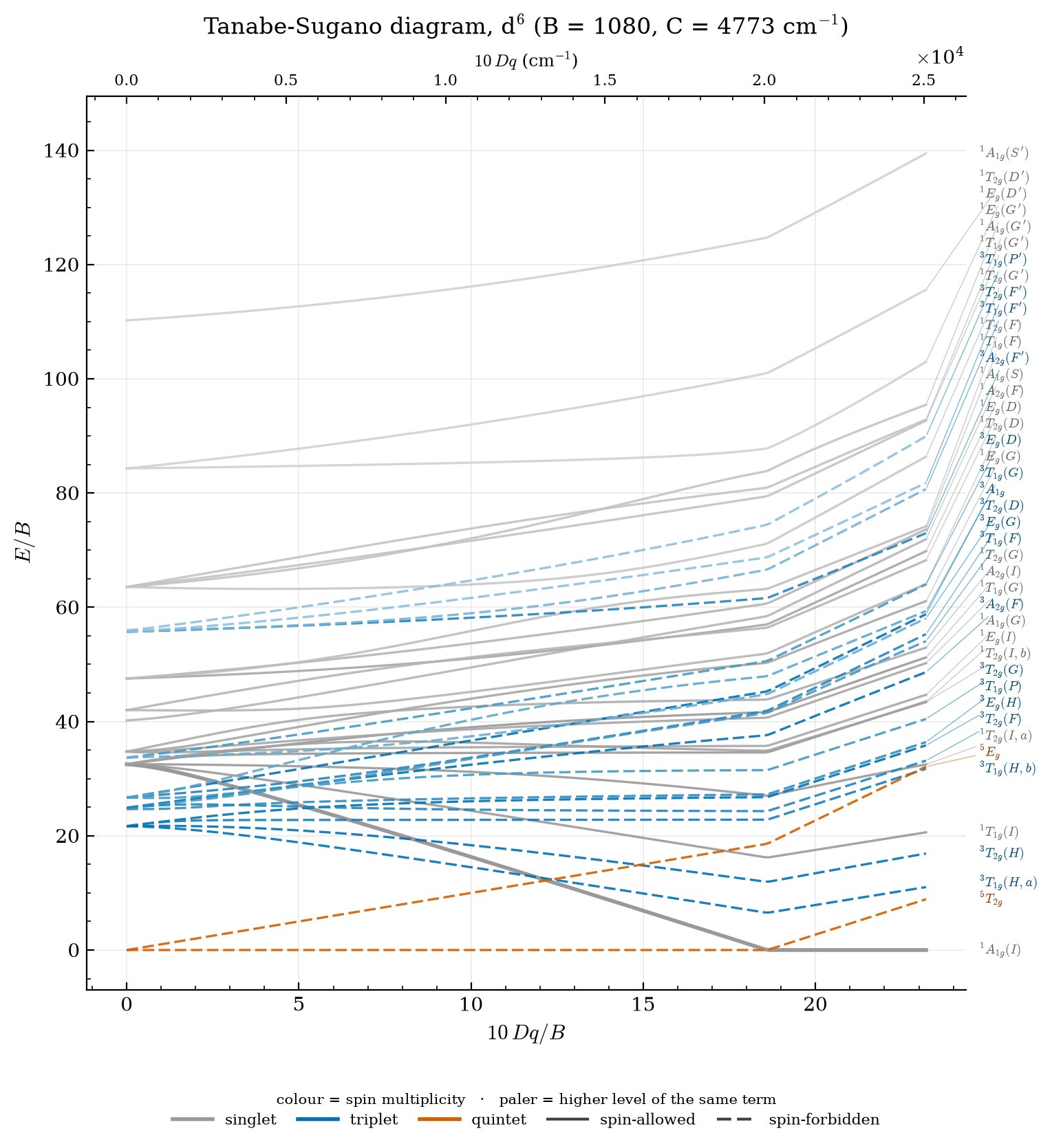
Figure: Tanabe-Sugano diagram (E/B vs 10Dq/B) showing energy levels normalized by the Racah B parameter
Energy-Correlation Diagram
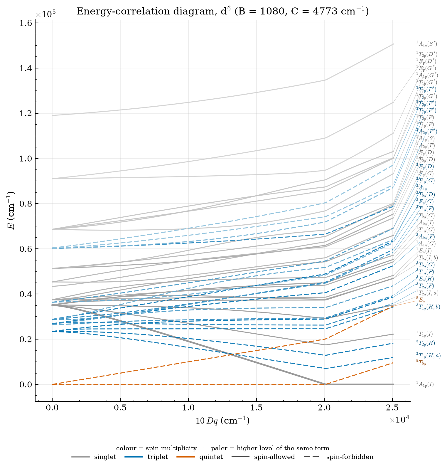
Figure: Energy-correlation diagram (E in cm⁻¹ vs 10Dq) showing absolute energy levels as a function of crystal field strength
Interactive Plotly Visualization
Interactive diagram for d6 with B = 1080 cm⁻¹ and C = 4773 cm⁻¹ — the same parameters as the static figures above, so the two can be read against each other:
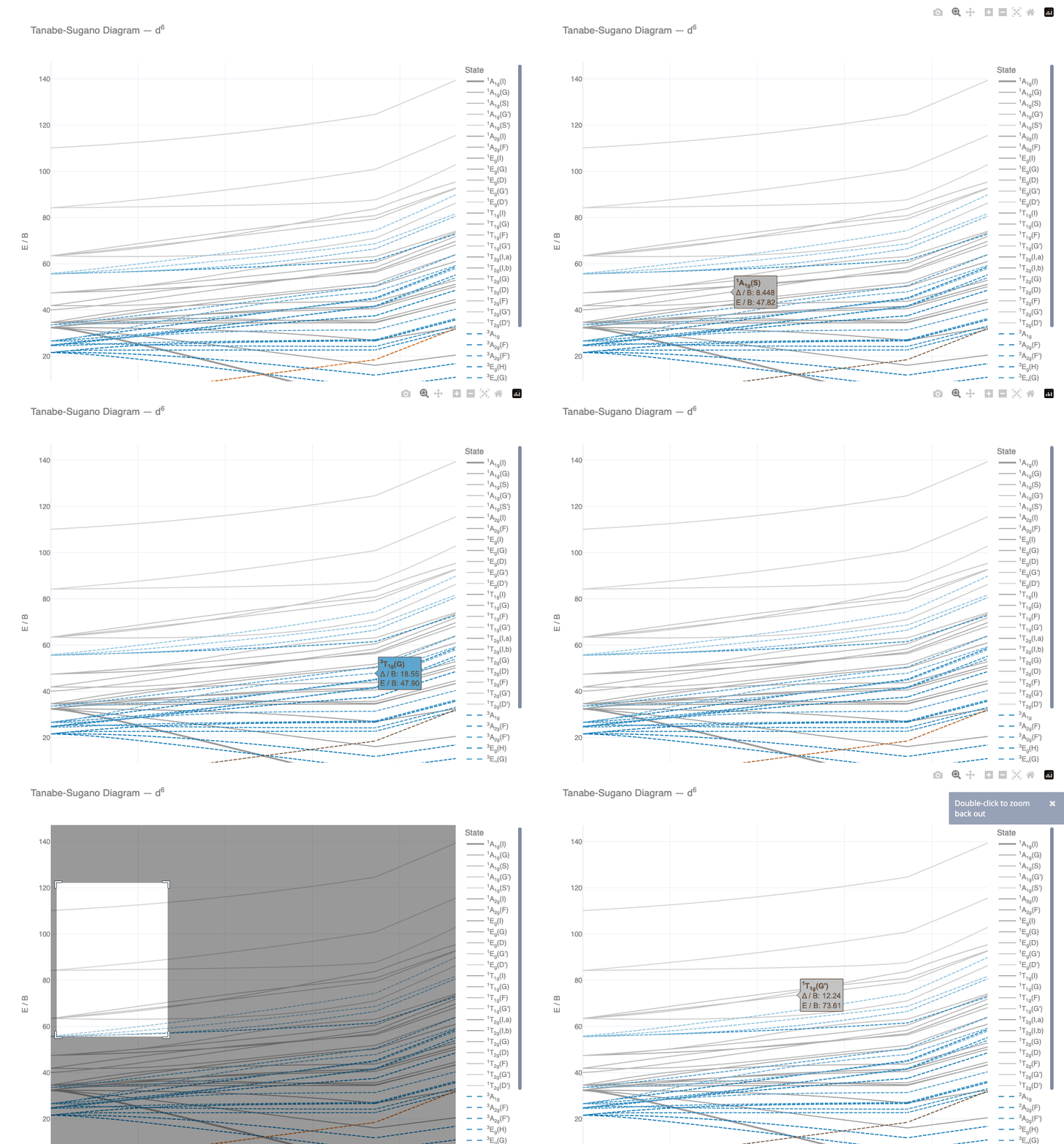
Figure: hover tooltips, legend isolation and drag-zoom. Recorded from the real
diagram by uv run poe regen-gif, not screen-captured
🌐 Interactive Diagrams
✨ NEW: Explore all Tanabe-Sugano diagrams online!
All diagrams (d² through d⁸) are now available on our interactive GitHub Pages site with full Plotly integration:
🔗 View Interactive Diagrams →
No installation required - just click and explore!
Every diagram is also committed as a static figure, so a paper or a slide deck does not need the browser:
| File | What it is |
|---|---|
ts-diagrams/d{N}/*.html |
Interactive Plotly diagram. References plotly.js from the CDN — run uv run poe regen-diagrams-offline, or pass -html -html-offline to the CLI, for a self-contained copy |
ts-diagrams/d{N}/*.png |
Publication-quality matplotlib raster (200 dpi) |
ts-diagrams/d{N}/*.pdf |
The same figure as vector, for a manuscript |
ts-diagrams/d{N}/*.csv |
Full-resolution eigenvalues (1000 sweep points) |
All four are regenerated by uv run poe regen-diagrams and guarded against
drift in CI. Both renderers read one palette and one notation ladder, so a state
is the same colour and carries the same symbol wherever you meet it:
- colour = spin multiplicity (Okabe-Ito, colour-blind safe)
- paler shade = higher level within the same term
- solid vs dashed = spin-allowed vs spin-forbidden from the ground level
🤖 MCP Server (Claude Desktop, Cursor, …)
TanabeSugano ships an optional Model Context Protocol server so AI assistants can compute diagrams, evaluate term symbols, and render plots as first-class tools.
Install
pip install "TanabeSugano[mcp]"
# or with uv:
uv add "TanabeSugano[mcp]"
Claude Desktop
Add to claude_desktop_config.json:
{
  "mcpServers": {
    "tanabesugano": {
      "command": "uvx",
      "args": ["--from", "tanabesugano[mcp]", "tanabesugano-mcp"]
    }
  }
}
One-click via .mcpb bundle
Every release attaches a tanabesugano-<version>.mcpb artifact (built by the Build .mcpb bundle job in cicd.yml) that Claude Desktop can install in one step — drag the file onto the Claude Desktop window. The bundle pins the exact published version and launches the tanabesugano-mcp entry point with the [mcp] extra; both are asserted by scripts/validate_mcpb.py before the release is created.
Exposed tools
Compute & analysis tools
| Tool | Description |
|---|---|
ts_supported_configs |
List supported d-configurations (d²–d⁸). |
ts_terms_table_data |
All eigenvalues at one (Dq, B, C), sorted ascending with multiplicity (machine-readable rows). |
ts_fit_spectrum |
Fit observed UV-Vis absorption peaks → Dq and Racah B. |
ts_nephelauxetic |
Interpret a fitted B as metal-ligand covalency (nephelauxetic β). |
ts_plot_png |
Matplotlib figure for any client. format="png" (default) returns an inline image; format="pdf" / "svg" return true vector output as an embedded resource — the only vector export route in the package. |
ts_fit_script |
Runnable matplotlib source for an observed-vs-computed fit figure. Carries the fitter's own numbers as literals and imports matplotlib only, so a reviewer can reproduce a published figure without installing this package. |
ts_plot_view |
Interactive Chart.js line plot (capable clients only). |
ts_explain |
One-paragraph ground-state description. |
ts_emit_png |
Internal export sink — each Chart.js iframe's "Send PNG to chat" button calls it with the rendered canvas. Not called directly. |
Note.
ts_computeandts_diagram(raw nested-dict eigenvalue payloads) were removed because the output was unusable without further rendering — Claude's "next steps" devolved into "save to CSV / render PNG" suggestions the client cannot execute. Usets_compute_app/ts_diagram_appfor in-chat tables and charts, orts_terms_table_datafor machine-readable rows.
Interactive app tools (Prefab / Chart.js UI — capable clients only)
| App | Description |
|---|---|
ts_dashboard_app |
Overview of all d²–d⁸ with ground terms, example ions, matrix sizes, and a concrete absorption-band number per configuration. |
ts_compute_app |
Sorted DataTable of every eigenvalue at one (Dq, B, C). Replaces the raw ts_compute. |
ts_diagram_app |
Full Tanabe-Sugano diagram as an interactive Chart.js line plot. |
ts_compare_app |
Multiple d-configurations overlaid on one shared Chart.js plot. |
ts_overlay_app |
Overlay multiple d-configurations on one shared chart. |
ts_oxidation_landscape_app |
Every eigenvalue of d²–d⁸ at fixed (Dq, B, C): style="scatter" (default) renders discrete dots per d-count, style="density" renders a Gaussian-broadened 2D heatmap (control σ via broadening_cm). |
ts_orgel_diagram_app |
Orgel diagram — E (cm⁻¹) vs Δ (cm⁻¹), the classic unnormalised companion to ts_diagram_app. d²/d³/d⁸ render smoothly; d⁴–d⁷ show the HS↔LS kink. |
ts_spin_crossover_app |
For d⁴/d⁵/d⁶/d⁷ only: ground-term energy of the candidate HS and LS curves vs Δ with the critical Dq annotated. Returns the numeric critical_Dq_cm1. |
ts_correlation_diagram_app |
Three-axis correlation diagram (free ion ↔ weak field ↔ strong field) — the classical Tsuchida/Cotton pedagogical bridge between free-ion term symbols and strong-field t₂g^x e_g^y configurations. |
ts_spectrum_app |
Simulated Lorentzian UV-Vis spectrum (spin-allowed + spin-forbidden). |
ts_reverse_fit_app |
Grid-search Dq and B to best-fit observed peak positions. |
ts_ratio_fit_app |
Derive Dq and B from 2–3 measured bands via the ratio method. |
ts_fit_plot_app |
Observed vs computed bands for a fit, plotted as residuals (computed − observed). A ~100 cm⁻¹ misfit is narrower than a marker on an 8,000–26,000 cm⁻¹ axis, so raw positions would show coincident dots; the raw values travel in the structured payload. |
Prompts & resources
Prompts: tanabesugano_why (discovery context) and tanabesugano_explain_complex (guided spectrum interpretation from measured absorption peaks).
Resources at tanabesugano://version, tanabesugano://configs, tanabesugano://config/{d} provide static metadata.
📚 Scientific Background
This implementation is based on the seminal work of Yukito Tanabe and Satoru Sugano:
📄 Original Publications
📖 Paper I: Absorption Spectra of Complex Ions
Authors: Yukito Tanabe, Satoru Sugano Journal: Journal of the Physical Society of Japan, Vol. 9, pp. 753-766 (1954) DOI: 10.1143/JPSJ.9.753 Link: https://journals.jps.jp/doi/10.1143/JPSJ.9.753
📖 Paper II: Absorption Spectra of Complex Ions
Authors: Yukito Tanabe, Satoru Sugano Journal: Journal of the Physical Society of Japan, Vol. 9, pp. 766-779 (1954) DOI: 10.1143/JPSJ.9.766 Link: https://journals.jps.jp/doi/10.1143/JPSJ.9.766
📖 Paper III: Calculation of Crystalline Field Strength
Authors: Yukito Tanabe, Satoru Sugano Journal: Journal of the Physical Society of Japan, Vol. 11, pp. 864-877 (1956) DOI: 10.1143/JPSJ.11.864 Link: https://journals.jps.jp/doi/10.1143/JPSJ.11.864
🤝 Contributing
We welcome contributions! Whether you're fixing bugs, adding features, or improving documentation, your help is appreciated.
- 📖 Read our Contributing Guide
- 🐛 Report issues on GitHub Issues
- 💡 Suggest features or improvements
- 🔧 Submit pull requests
📝 Citation
If you use TanabeSugano in your research, please cite:
@software{tanabesugano,
  author       = {Hahn, Anselm W.},
  title        = {TanabeSugano: Python-based Eigensolver for Tanabe-Sugano Diagrams},
  year         = {2026},
  publisher    = {Zenodo},
  version      = {2.0.0-alpha.1},
  doi          = {10.5281/zenodo.3402463},
  url          = {https://github.com/Anselmoo/TanabeSugano}
}
Which DOI?
10.5281/zenodo.3402463is the concept DOI — it always resolves to the newest deposited release, which is what you want in a reference list. To cite the exact version you ran, use that release's own version DOI from the Zenodo record instead.
📄 License
This project is licensed under the MIT License - see the LICENSE file for details.
Made with ❤️ for the scientific community
⭐ Star us on GitHub — it helps!
1 maintainer

Metadata
1 maintainer
Release files for tanabesugano 2.0.0
For a detailed explanation of source distributions (sdists) and built distributions (wheels), please see the package formats documentation.
Source distribution (sdist)
| File | Size | Uploaded | |
|---|---|---|---|
| tanabesugano-2.0.0.tar.gz | 227.0 kB | Details |
Built distribution (wheel)
| File | Interpreter | ABI | Platform | Reset |
|---|---|---|---|---|
| tanabesugano-2.0.0-py3-none-any.whl | Python 3 | none | any | Details |
Total release size: 475.7 kB
Release files / tanabesugano-2.0.0.tar.gz
| Download URL | tanabesugano-2.0.0.tar.gz |
|---|---|
| Size | 227.0 kB |
| Tags | Source |
|
SHA-256 checksum How to use checksums |
1bfbf13ad7af744cf58fe2ff6443075a52902669f07f58fcc2f283c31f188e19
|
|
BLAKE2b-256 checksum How to use checksums |
0d268e64b25e4b4455f08afc6ee066031ea5c4c4ad6648fbef12459f902268af
|
| Upload date | |
|
Uploaded using Trusted Publishing? What is trusted publishing? |
Yes |
| Uploaded via |
twine/7.0.0 CPython/3.13.14
|
Provenance
Provenance describes where a file came from. On PyPI, provenance is shared via attestations, which provide a verifiable record of the build or publishing details. View details, limitations and caveats.


PyPI Publish Attestation
PyPI verified that this artifact, at this checksum, originated from the publisher listed below.
Signed by GitHub Actions, verified by PyPI on Aug 23, 2026.
Transparency logRelease files / tanabesugano-2.0.0-py3-none-any.whl
| Download URL | tanabesugano-2.0.0-py3-none-any.whl |
|---|---|
| Size | 248.7 kB |
| Tags | Python 3 |
|
SHA-256 checksum How to use checksums |
dcf53d99dc69429350690c4b167248d2e1d3dea0741a3d44009c798eca0629ff
|
|
BLAKE2b-256 checksum How to use checksums |
a43d44f97e9a67e74faf2208821575c58998ff61b3936c80169cdf17a9097311
|
| Upload date | |
|
Uploaded using Trusted Publishing? What is trusted publishing? |
Yes |
| Uploaded via |
twine/7.0.0 CPython/3.13.14
|
Provenance
Provenance describes where a file came from. On PyPI, provenance is shared via attestations, which provide a verifiable record of the build or publishing details. View details, limitations and caveats.
PyPI Publish Attestation
PyPI verified that this artifact, at this checksum, originated from the publisher listed below.
Signed by GitHub Actions, verified by PyPI on Aug 23, 2026.
Transparency log













