No project description provided

Project description
TDAvec.py
TDAvec.py is a python interface to TDAvec R package, which is available on CRAN
First of all, it allows access to all implemented in the original R package vectorizations functions:
- computeAlgebraicFunctions: Compute Algebraic Functions from a Persistence Diagram
- computeBettiCurve: A Vector Summary of the Betti Curve
- computeComplexPolynomial: Compute Complex Polynomial Coefficients from a Persistence Diagram
- computeEulerCharacteristic: A Vector Summary of the Euler Characteristic Curve
- computeNormalizedLife: A Vector Summary of the Normalized Life Curve
- computePersistenceBlock: A Vector Summary of the Persistence Block
- computePersistenceImage: A Vector Summary of the Persistence Surface
- computePersistenceLandscape: Vector Summaries of the Persistence Landscape Functions
- computePersistenceSilhouette: A Vector Summary of the Persistence Silhouette Function
- computePersistentEntropy: A Vector Summary of the Persistent Entropy Summary Function
- computeStats: Compute Descriptive Statistics for Births, Deaths, Midpoints, and Lifespans in a Persistence Diagram
- computeTemplateFunction: Compute a Vectorization of a Persistence Diagram based on Tent Template Functions
- computeTropicalCoordinates: Compute Tropical Coordinates from a Persistence Diagram
All these functions can easily be called using tdavec.tdavec_core package.
In addition, we provide also sklearn-type interface to the same functionality, which could be more familiar for python programmers.
Note that the package was tested only on python 3.12.
Setup
TDAvec.py is available on pypi. To install it simply type
pip install tdavec
into your environment.
You can also install the current verion from the GitHub with
pip install -e "git+https://github.com/uislambekov/TDAvec.git#egg=tdavec&subdirectory=python"
Alternatively, you can install it from the source. In order to do this clone mentioned above github repository and run the followin commants from the project root directory:
pip install numpy==1.26.4 ripser==0.6.8
python3 setup.py build_ext --inplace
pip install .
after that you should have tdavec package installed in your environment.
In order to check if the intallation process was completed, you can run python and evaluate the following lines:
> from tdavec import test_package
> X, D, PS = test_package()
This function will create a simple point cloud, build a persistence diagram, caclulate the Persistence Silhouette vectorization from it, and return these three objects.
Usage
In this section some simple example of package usage is demonstrated.
We will start with loading TDAvec library and some other packages:
from tdavec import createEllipse, TDAvectorizer, tdavec_core
import matplotlib.pyplot as plt
from sklearn.linear_model import LinearRegression
from sklearn.model_selection import train_test_split
from sklearn.metrics import mean_squared_error
import pandas as pd
import numpy as np
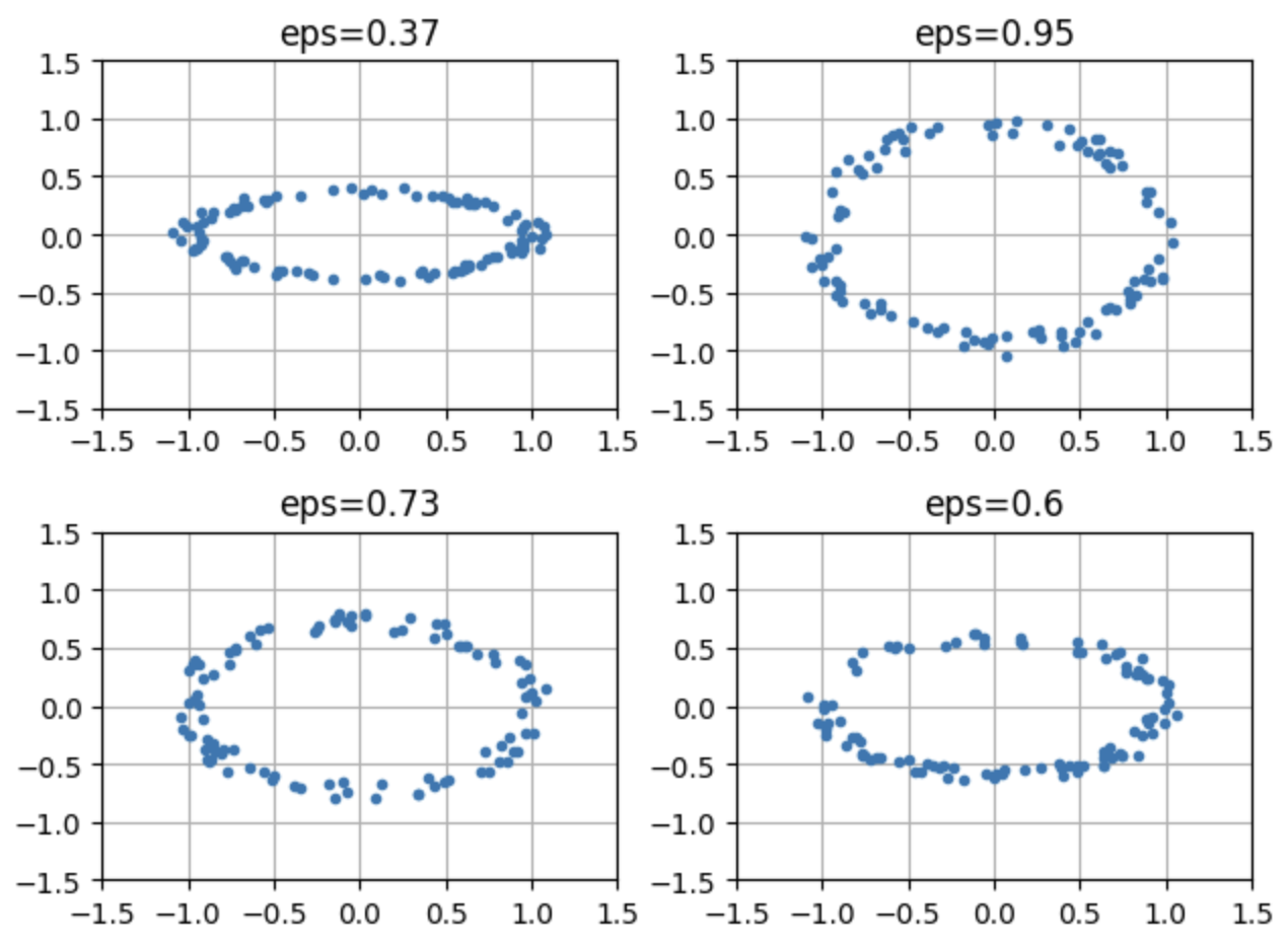
As a sample data we will work with set of point clouds, that represent defomed elipses with randomly selected squize rations:
np.random.seed(42)
epsList = np.random.uniform(low = 0, high = 1, size = 500)
clouds = [createEllipse(a=1, b=eps, n=100) for eps in epsList]
Here are some examples:
for i, cl in enumerate(clouds[:4]):
    plt.subplot(2, 2, i+1)
    plt.plot(cl[:,0], cl[:,1], ".")
    plt.xlim(-1.5, 1.5); plt.ylim(-1.5, 1.5)
    plt.title(f"eps={np.round(epsList[i], 2)}")
    plt.grid()
plt.tight_layout()
In order to generate Persistence Diagrams one need to create TDAvectorizer object and fit fit it:
v = TDAvectorizer()
v.setParams({"scale":np.linspace(0, 2, 10)})
v.fit(clouds)
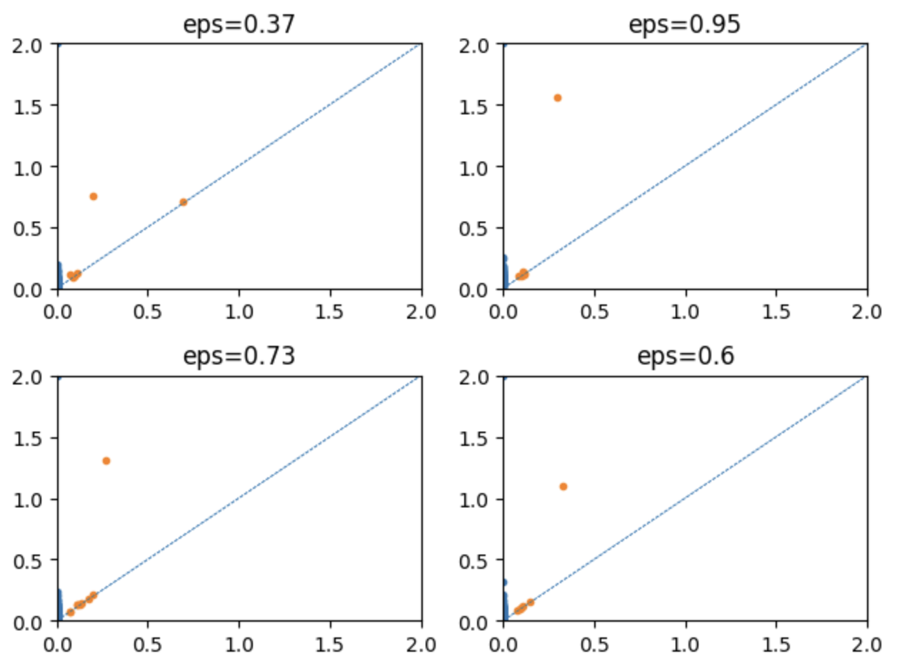
Here are the examples of the generated persistence diagrams:
for i in range(4):
    plt.subplot(2,2,i+1)
    PD = v.diags[i]
    for dim in range(2):
        plt.plot(PD[dim][:,0], PD[dim][:,1], ".")
        plt.xlim(0, 2); plt.ylim(0, 2)
        plt.axline( (0,0), slope = 1, linestyle = "--", linewidth = 0.5)
        plt.title(f"eps={np.round(epsList[i], 2)}")
plt.tight_layout()
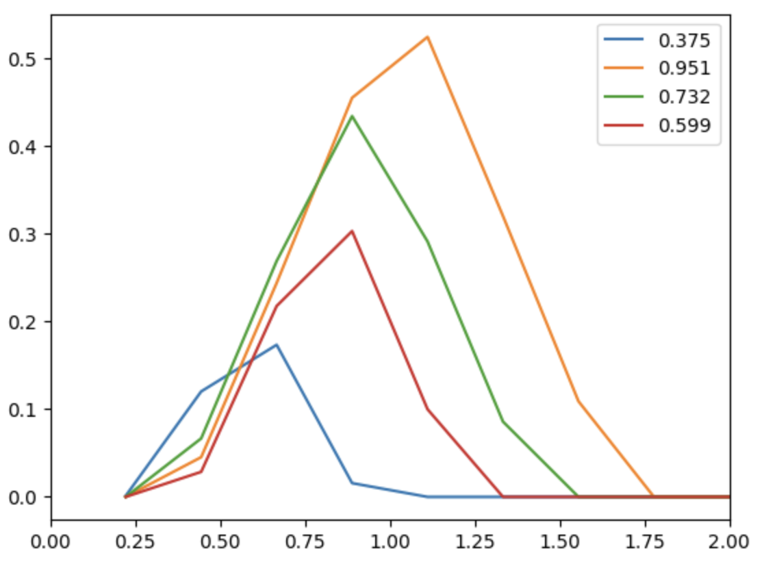
Once TDAvectorizer object is fitted, one can calculate vectorization by calling transorm() method of this object:
X = v.transform(output="PS", homDim=1)
for i, e in enumerate(epsList[:4]):
    plt.plot(v.getParams()["scale"][1:],X[i,:], label=np.round(e, 3))
    plt.xlim(0, 2)
plt.legend()
plt.show()
These vectorizations can be used as predictors for ML problem, whose goal is to predict the original deformation parameter. We will use a simple sklearn.LinearRegression model to solve the problem
Here is a simple function the for any given set of predictors creates the model, solves it, and retirns the results:
def makeSim(X, y=epsList):
    Xtrain, Xtest, ytrain, ytest = train_test_split(X, y, train_size=0.8, random_state=42)
    model = LinearRegression().fit(Xtrain, ytrain)
    test_preds = model.predict(Xtest)
    score = model.score(Xtest, ytest)
    res = {"method":method, "homDim":homDim, "test_preds":test_preds, "y_test":ytest, "score":score}
    return res
In the loop below a systematic scan over different vectorizattion methods and homological dimensions is performed:
v.setParams({"scale":np.linspace(0, 2, 30)})
methodList = v.vectorization_names
results = []
df = pd.DataFrame()
for homDim in [0, 1]:
    print(f" Dimension {homDim}: ", end=" ")
    for method in methodList[:-2]:
        print(method, end = " ")
        X =v.transform(output=method, homDim=homDim)
        res = makeSim(X); results.append(res)
        df = pd.concat([df, pd.DataFrame(res)])
    print()
Here is the table of calculated accuracies:
| method/dimension | 0 | 1 |
|---|---|---|
| ecc | 0.976 | 0.996 |
| vab | 0.976 | 0.986 |
| fda | 0.983 | 0.985 |
| nl | 0.96 | 0.981 |
| poly | 0.967 | 0.975 |
| algebra | 0.971 | 0.955 |
| ps | 0.946 | 0.914 |
| stats | 0.987 | 0.887 |
| pes | 0.989 | 0.717 |
| pi | 0.986 | 0.547 |
As you can see, majority off them are very close to 1, which means that the models are pretty accurate. Presented belowe truth/predictions scatter plots confirm this conslusion:

Release history Release notifications | RSS feed


Download files
Download the file for your platform. If you're not sure which to choose, learn more about installing packages.
Source Distribution
Built Distribution
Filter files by name, interpreter, ABI, and platform.
If you're not sure about the file name format, learn more about wheel file names.
Copy a direct link to the current filters
File details
Details for the file tdavec-0.1.5.tar.gz.
File metadata
- Download URL: tdavec-0.1.5.tar.gz
- Upload date:
- Size: 265.1 kB
- Tags: Source
- Uploaded using Trusted Publishing? No
- Uploaded via: twine/6.1.0 CPython/3.11.13
File hashes
| Algorithm | Hash digest | |
|---|---|---|
| SHA256 |
249e780baa965317194d411f0eb1efe0dca0b264709749686644385d84d4fe32
|
|
| MD5 |
6405664fa3a04a642613fa87de34d9ee
|
|
| BLAKE2b-256 |
aaa31313ae5d6da8574817c9258f3ed11bd01d752e5196f84825984b54514e48
|
File details
Details for the file tdavec-0.1.5-cp311-cp311-macosx_10_13_x86_64.whl.
File metadata
- Download URL: tdavec-0.1.5-cp311-cp311-macosx_10_13_x86_64.whl
- Upload date:
- Size: 462.2 kB
- Tags: CPython 3.11, macOS 10.13+ x86-64
- Uploaded using Trusted Publishing? No
- Uploaded via: twine/6.1.0 CPython/3.11.13
File hashes
| Algorithm | Hash digest | |
|---|---|---|
| SHA256 |
00c456582da7161c13d5f6730d702afa23d6dd74587386a5805daf817e5ed4c2
|
|
| MD5 |
d15372c793cfee3540c1e5bfc6266d1e
|
|
| BLAKE2b-256 |
5dbd796aed448f1f99108f293da9db4161ad95cb37d1282f931b72f9d3d518ca
|


