

Differentiable Tensors based on NumPy Arrays.







Highlights
- Write differentiable code with Tensors based on NumPy arrays
- Forward Mode Automatic Differentiation (AD) using Hyper-Dual Tensors, up to second order derivatives
- Efficient evaluation of batches by elementwise-operating trailing axes
- Essential vector/tensor Hyper-Dual number math, including limited support for
einsum(restricted to max. four operands) - Math is limited but similar to NumPy, try to use
import tensortrax.math as tminstead ofimport numpy as npinside functions to be differentiated - Create functions in terms of Hyper-Dual Tensors
- Evaluate the function, the gradient (jacobian) and the hessian of scalar-valued functions or functionals on given input arrays
- Straight-forward definition of custom functions in variational-calculus notation
- Stable gradient and hessian of eigenvalues obtained from
eigvalshin case of repeated equal eigenvalues
Motivation
Gradient and hessian evaluations of functions or functionals based on tensor-valued input arguments are a fundamental repetitive and (error-prone) task in constitutive hyperelastic material formulations used in continuum mechanics of solid bodies. In the worst case, conceptual ideas are impossible to pursue because the required tensorial derivatives are not readily achievable. The Hyper-Dual number approach enables a generalized and systematic way to overcome this deficiency [2]. Compared to existing Hyper-Dual Number libaries ([3], [4]) which introduce a new (hyper-) dual dtype (treated as dtype=object in NumPy), tensortrax relies on its own Tensor class. This approach involves a re-definition of all essential math operations (and NumPy-functions), whereas the dtype-approach supports most basic math operations out of the box. However, in tensortrax NumPy and all its underlying linear algebra functions operate on default data types (e.g. dtype=float). This allows to support functions like np.einsum(). Beside the differences concerning the underlying dtype, tensortrax is formulated on easy-to-understand (tensorial) calculus of variation. Hence, gradient- and hessian-vector products are evaluated with very little overhead compared to analytic formulations.
Installation
Install tensortrax from PyPI, the Python Package Index.
pip install tensortrax[all]
tensortrax has minimal requirements, all available at PyPI.
To install optional dependencies as well, add [all] to the install command: pip install tensortrax[all].
scipyfor extended math-support
Usage
Let's define a scalar-valued function which operates on a tensor. The math module tensortrax.math provides some essential NumPy-like functions including linear algebra.
import tensortrax as tr
import tensortrax.math as tm


def fun(F, mu=1):
    C = F.T @ F
    I1 = tm.trace(C)
    J = tm.linalg.det(F)
    return mu / 2 * (J ** (-2 / 3) * I1 - 3)
The Hessian of the scalar-valued function w.r.t. the chosen function argument (here, wrt=0 or wrt="F") is evaluated by variational calculus (Forward Mode AD implemented as Hyper-Dual Tensors). The function is called once for each component of the hessian (symmetry is taken care of). The function and the gradient are evaluated with no additional computational cost. Optionally, the function, gradient and Hessian calls are executed in parallel (threaded).
import numpy as np

# some random input data
np.random.seed(125161)
F = (np.eye(3) + np.random.rand(50, 8, 3, 3) / 10).T

# W = tr.function(fun, wrt=0, ntrax=2)(F)
# dWdF = tr.gradient(fun, wrt=0, ntrax=2)(F)
# d2WdF2, dWdF, W = tr.hessian(fun, wrt="F", ntrax=2, full_output=True)(F=F)
d2WdF2 = tr.hessian(fun, wrt="F", ntrax=2, parallel=False)(F=F)
Another possibility is to define and operate on Tensors manually. This enables more flexible coding, which wouldn't be possible with the builtin functions. The Hu-Washizu Three-Field-Variational principle for nearly incompressible hyperelastic solids [5] is used here to obtain mixed partial derivatives. Some random input arrays are generated and a Tensor is created for each variable. After performing some math, the hessian of the resulting tensor object is extracted.
# some random input data
n = 10
x = (np.eye(3) + np.random.rand(n, 3, 3) / 10).T
y = np.random.rand(n)
z = np.random.rand(n) / 10 + 1

# create tensors
F = tr.Tensor(x, ntrax=1)
p = tr.Tensor(y, ntrax=1)
J = tr.Tensor(z, ntrax=1)


def neo_hooke(F, mu=1):
    "Strain energy function of the Neo-Hookean material formulation."
    C = F.T @ F
    I3 = tm.linalg.det(C)
    return mu * (I3 ** (-1 / 3) * tm.trace(C) - 3) / 2


def volumetric(J, bulk=20):
    "Volumetric strain energy function."
    return bulk * (J - 1) ** 2 / 2


def W(F, p, J):
    "Hu-Washizu (u, p, J) - Three-Field-Variation."
    detF = tm.linalg.det(F)
    return neo_hooke(F) + volumetric(J) + p * (detF - J)


# init Tensors to be used with second partial derivatives
F.init(hessian=True, δx=False, Δx=False)
p.init(hessian=True, δx=True, Δx=False)
J.init(hessian=True, δx=False, Δx=True)

# evaluate a mixed second partial derivative
dWdpdJ = tr.Δδ(W(F, p, J))
In a similar way, the gradient may be obtained by initiating a Tensor with the gradient argument.
# init Tensors to be used with first partial derivatives
F.init(gradient=True, δx=False)
p.init(gradient=True, δx=True)
J.init(gradient=True, δx=False)

# evaluate a partial derivative
dWdp = tr.δ(W(F, p, J))
Performance
A benchmark for the gradient and hessian runtimes of an isotropic hyperelastic strain energy function demonstrates the performance of this package compared to Autograd [1]. The hessian is evaluated in about 2.5 seconds for one million input tensors (Intel Core i7-11850H, 32GB RAM). While the runtimes of the gradients evaluated by Tensortrax are similar compared to those of Autograd, the Hessian evaluation in Tensortrax is much faster than in Autograd (see Table 1, Table 2 and Figure 1). Note that this is only one exemplaric benchmark for a specific kind of function - runtimes may vary.
\psi(\boldsymbol{C}) = tr(\boldsymbol{C}) - \ln(\det(\boldsymbol{C}))
Table 1: Runtimes of Gradients evaluated by tensortrax and autograd.
| Tensors | Gradient (Tensortrax) in s | Gradient (Autograd) in s | Speedup |
|---|---|---|---|
| 1 | 0.00071 | 0.00082 | x 1.16 |
| 4 | 0.00075 | 0.00070 | x 0.93 |
| 16 | 0.00075 | 0.00071 | x 0.94 |
| 64 | 0.00083 | 0.00077 | x 0.94 |
| 256 | 0.00097 | 0.00094 | x 0.97 |
| 1024 | 0.00160 | 0.00161 | x 1.01 |
| 4096 | 0.00568 | 0.00428 | x 0.75 |
| 16384 | 0.01233 | 0.01690 | x 1.37 |
| 65536 | 0.06103 | 0.06756 | x 1.11 |
| 262144 | 0.27910 | 0.26911 | x 0.96 |
| 1048576 | 1.15561 | 1.09512 | x 0.95 |
Table 2: Runtimes of Hessians evaluated by tensortrax and autograd.
| Tensors | Hessian (Tensortrax) in s | Hessian (Autograd) in s | Speedup |
|---|---|---|---|
| 1 | 0.00068 | 0.01348 | x 19.77 |
| 4 | 0.00073 | 0.00723 | x 9.87 |
| 16 | 0.00076 | 0.00718 | x 9.41 |
| 64 | 0.00083 | 0.00792 | x 9.58 |
| 256 | 0.00111 | 0.01044 | x 9.43 |
| 1024 | 0.00214 | 0.02094 | x 9.79 |
| 4096 | 0.00844 | 0.06148 | x 7.28 |
| 16384 | 0.02544 | 0.23778 | x 9.35 |
| 65536 | 0.11685 | 0.95208 | x 8.15 |
| 262144 | 0.51561 | 3.94024 | x 7.64 |
| 1048576 | 2.13629 | 16.15154 | x 7.56 |
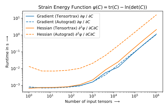
Figure 1: Runtime vs. Number of input tensors - plot for Gradients and Hessians evaluated by tensortrax and autograd.
Theory
The calculus of variation deals with variations, i.e. small changes in functions and functionals. A small-change in a function is evaluated by applying small changes on the tensor components.
\psi = \psi(\boldsymbol{F})
\delta \psi = \delta \psi(\boldsymbol{F}, \delta \boldsymbol{F})
Let's take the trace of a tensor product as an example. The variation is evaluated as follows:
\psi = tr(\boldsymbol{F}^T \boldsymbol{F}) = \boldsymbol{F} : \boldsymbol{F}
\delta \psi = \delta \boldsymbol{F} : \boldsymbol{F} + \boldsymbol{F} : \delta \boldsymbol{F} = 2 \ \boldsymbol{F} : \delta \boldsymbol{F}
The $P_{ij}$ - component of the jacobian $\boldsymbol{P}$ is now numerically evaluated by setting the respective variational component $\delta F_{ij}$ of the tensor to one and all other components to zero. In total, $i \cdot j$ function calls are necessary to assemble the full jacobian. For example, the $12$ - component is evaluated as follows:
\delta \boldsymbol{F}_{(12)} = \begin{bmatrix} 0 & 1 & 0 \\ 0 & 0 & 0 \\ 0 & 0 & 0 \end{bmatrix}
\delta_{(12)} \psi = \frac{\partial \psi}{\partial F_{12}} = 2 \ \boldsymbol{F} : \delta \boldsymbol{F}_{(12)} = 2 \ \boldsymbol{F} : \begin{bmatrix} 0 & 1 & 0 \\ 0 & 0 & 0 \\ 0 & 0 & 0 \end{bmatrix}
The second order variation, i.e. a variation applied on another variation of a function is evaluated in the same way as a first order variation.
\Delta \delta \psi = 2 \ \delta \boldsymbol{F} : \Delta \boldsymbol{F} + 2 \ \boldsymbol{F} : \Delta \delta \boldsymbol{F}
Once again, each component $A_{ijkl}$ of the fourth-order hessian is numerically evaluated. In total, $i \cdot j \cdot k \cdot l$ function calls are necessary to assemble the full hessian (without considering symmetry). For example, the $1223$ - component is evaluated by setting $\Delta \delta \boldsymbol{F} = \boldsymbol{0}$ and $\delta \boldsymbol{F}$ and $\Delta \boldsymbol{F}$ as follows:
\delta \boldsymbol{F}_{(12)} = \begin{bmatrix} 0 & 1 & 0 \\ 0 & 0 & 0 \\ 0 & 0 & 0 \end{bmatrix}
\Delta \boldsymbol{F}_{(23)} = \begin{bmatrix} 0 & 0 & 0 \\ 0 & 0 & 1 \\ 0 & 0 & 0 \end{bmatrix}
\Delta \delta \boldsymbol{F} = \begin{bmatrix} 0 & 0 & 0 \\ 0 & 0 & 0 \\ 0 & 0 & 0 \end{bmatrix}
\Delta_{(23)} \delta_{(12)} \psi = \Delta_{(12)} \delta_{(23)} \psi = \frac{\partial^2 \psi}{\partial F_{12}\ \partial F_{23}}
\Delta_{(23)} \delta_{(12)} \psi = 2 \ \delta \boldsymbol{F}_{(12)} : \Delta \boldsymbol{F}_{(23)} + 2 \ \boldsymbol{F} : \Delta \delta \boldsymbol{F}
Numeric calculus of variation in tensortrax
Each Tensor has four attributes: the (real) tensor array and the (hyper-dual) variational arrays. To obtain the above mentioned $12$ - component of the gradient and the $1223$ - component of the hessian, a tensor has to be created with the appropriate small-changes of the tensor components (dual arrays).
import tensortrax as tr
from tensortrax import Tensor, f, δ, Δ, Δδ
from tensortrax.math import trace

δF_12 = np.array(
    [
        [0, 1, 0],
        [0, 0, 0],
        [0, 0, 0],
    ],
    dtype=float,
)

ΔF_23 = np.array(
    [
        [0, 0, 0],
        [0, 0, 1],
        [0, 0, 0],
    ],
    dtype=float,
)

x = np.eye(3) + np.arange(9).reshape(3, 3) / 10
F = Tensor(x=x, δx=δF_12, Δx=ΔF_23, Δδx=None)
I1_C = trace(F.T @ F)
The function as well as the gradient and hessian components are accessible as:
ψ = f(I1_C)
P_12 = δ(I1_C)  # (= Δ(I1_C))
A_1223 = Δδ(I1_C)
To obtain full gradients and hessians of scalar-valued functions in one function call, tensortrax provides helpers (decorators) which handle the multiple function calls.
fun = lambda F: trace(F.T @ F)

func = tr.function(fun)(x)
grad = tr.gradient(fun)(x)
hess = tr.hessian(fun)(x)
For tensor-valued functions, use jacobian() instead of gradient().
fun = lambda F: F.T @ F

jac = tr.jacobian(fun)(x)
Evaluate the gradient- as well as the hessian-vector(s)-product:
gvp = tr.gradient_vector_product(fun)(x, δx=x)
hvp = tr.hessian_vector_product(fun)(x, δx=x)
hvsp = tr.hessian_vectors_product(fun)(x, δx=x, Δx=x)
Extensions
Custom functions (extensions) are easy to implement in tensortrax. Beside the function expression, three additional (dual) variation expressions have to be defined.
import numpy as np
from tensortrax import Tensor, f, δ, Δ, Δδ


def sin(A):
    return Tensor(
        x=np.sin(f(A)),
        δx=np.cos(f(A)) * δ(A),
        Δx=np.cos(f(A)) * Δ(A),
        Δδx=-np.sin(f(A)) * δ(A) * Δ(A) + np.cos(f(A)) * Δδ(A),
        ntrax=A.ntrax,
    )


x = np.eye(3)
y = sin(Tensor(x))
Contributors
 Andreas Dutzler 💻 💡 📖 🤔 |
 Mohamed ZAARAOUI 🤔 |
References
- D. Maclaurin, D. Duvenaud, M. Johnson and J. Townsend, Autograd. [Online]. Available: https://github.com/HIPS/autograd.
- J. Fike and J. Alonso, The Development of Hyper-Dual Numbers for Exact Second-Derivative Calculations, 49th AIAA Aerospace Sciences Meeting including the New Horizons Forum and Aerospace Exposition. American Institute of Aeronautics and Astronautics, Jan. 04, 2011,
.
- P. Rehner and G. Bauer, Application of Generalized (Hyper-) Dual Numbers in Equation of State Modeling, Frontiers in Chemical Engineering, vol. 3, 2021. Available: https://github.com/itt-ustutt/num-dual.
- T. Oberbichler, HyperJet. [Online]. Available: http://github.com/oberbichler/HyperJet.
- J. Bonet and R. D. Wood, Nonlinear Continuum Mechanics for Finite Element Analysis, 2nd ed. Cambridge: Cambridge University Press, 2008,
.
1 maintainer

Metadata
1 maintainer
Release files for tensortrax 0.28.0
For a detailed explanation of source distributions (sdists) and built distributions (wheels), please see the package formats documentation.
Source distribution (sdist)
| File | Size | Uploaded | |
|---|---|---|---|
| tensortrax-0.28.0.tar.gz | 78.4 kB | Details |
Built distribution (wheel)
| File | Interpreter | ABI | Platform | Reset |
|---|---|---|---|---|
| tensortrax-0.28.0-py3-none-any.whl | Python 3 | none | any | Details |
Total release size: 133.7 kB
Release files / tensortrax-0.28.0.tar.gz
| Download URL | tensortrax-0.28.0.tar.gz |
|---|---|
| Size | 78.4 kB |
| Tags | Source |
|
SHA-256 checksum How to use checksums |
c63504ae9fb619b4936bf95d8404d9b7677810d2b159d878665cbf25ef77efe1
|
|
BLAKE2b-256 checksum How to use checksums |
7738d173c33b88e03ac841ad861cf7bd9d6a548fad196e16ec420c63e7b949ea
|
| Upload date | |
|
Uploaded using Trusted Publishing? What is trusted publishing? |
No |
| Uploaded via |
twine/7.0.0 CPython/3.13.14
|
Release files / tensortrax-0.28.0-py3-none-any.whl
| Download URL | tensortrax-0.28.0-py3-none-any.whl |
|---|---|
| Size | 55.3 kB |
| Tags | Python 3 |
|
SHA-256 checksum How to use checksums |
ab87bf1660b07092cdac1378523e05a60c81648d270bab35026647e4e0778c48
|
|
BLAKE2b-256 checksum How to use checksums |
b881631bb16821a0b8cf85feb6af7a39db37447d49c9401805fa43191f9fe84b
|
| Upload date | |
|
Uploaded using Trusted Publishing? What is trusted publishing? |
No |
| Uploaded via |
twine/7.0.0 CPython/3.13.14
|














