Tensorflow implementation of Levenberg-Marquardt training algorithm

Project description
Tensorflow Levenberg-Marquardt

Implementation of Levenberg-Marquardt training for models that inherits from tf.keras.Model. The algorithm has been extended to support mini-batch training for both regression and classification problems.
A PyTorch implementation is also available: torch-levenberg-marquardt
Implemented losses
- MeanSquaredError
- ReducedOutputsMeanSquaredError
- CategoricalCrossentropy
- SparseCategoricalCrossentropy
- BinaryCrossentropy
- SquaredCategoricalCrossentropy
- CategoricalMeanSquaredError
- Support for custom losses
Implemented damping algorithms
Implemented damping algorithms
- Standard: $\large J^T J + \lambda I$
- Fletcher: $\large J^T J + \lambda ~ \text{diag}(J^T J)$
- Support for custom damping algorithm
More details on Levenberg-Marquardt can be found on this page.
Usage
Suppose that model and train_dataset has been created, it is possible to train the model in two different ways.
Custom Model.fit
This is similar to the standard way models are trained with keras, the difference is that the fit method is called on a ModelWrapper class instead of calling it directly on the model class.
import tf_levenberg_marquardt as lm

model_wrapper = lm.model.ModelWrapper(model)

model_wrapper.compile(
    optimizer=tf.keras.optimizers.SGD(learning_rate=0.1),
    loss=lm.loss.SparseCategoricalCrossentropy(from_logits=True),
    metrics=['accuracy'])

model_wrapper.fit(train_dataset, epochs=5)
Custom training loop
This alternative is less flexible than Model.fit as for example it does not support callbacks and is only trainable using tf.data.Dataset.
import levenberg_marquardt as lm

trainer = lm.training.Trainer(
    model=model,
    optimizer=tf.keras.optimizers.SGD(learning_rate=0.1),
    loss=lm.loss.SparseCategoricalCrossentropy(from_logits=True))

trainer.fit(
    dataset=train_dataset,
    epochs=5,
    metrics=[tf.keras.metrics.SparseCategoricalAccuracy()])
Memory, Speed and Convergence considerations
In order to achieve the best performances out of the training algorithm some considerations have to be done, so that the batch size and the number of weights of the model are chosen properly. The Levenberg-Marquardt algorithm is used to solve the least squares problem
$\large (1)$
$$ \large \underset{W}{\text{argmin}} \sum_{i=1}^{N} [y_i - f(x_i, W)]^2 $$
where $\large y_i - f(x_i, w)$ are the residuals, $\large W$ are weights of the model and $\large N$ the number of residuals, which can be obtained by multiplying the batch size with the number of outputs of the model.
$\large (2)$
$$ \large \text{num\_residuals} = \text{batch\_size} \cdot \text{num\_outputs} $$
The Levenberg-Marquardt updates can be computed using two equivalent formulations
$\large (3\text{a})$
$$ \large \text{updates} = (J^T J + \text{damping})^{-1} J^T \text{residuals} $$
$\large (3\text{b})$
$$ \large \text{updates} = J^T (JJ^T + \text{damping})^{-1} \text{residuals} $$
given that the size of the jacobian matrix is [num_residuals x num_weights]. In the first equation $\large (J^T J + \text{damping})$ have size [num_weights x num_weights], while in the second equation $\large (JJ^T + \text{damping})$ have size [num_residuals x num_residuals]. The first equation is convenient when num_residuals > num_weights overdetermined, while the second equation is convenient when num_residuals < num_weights underdetermined. For each batch the algorithm checks whether the problem is overdetermined or underdetermined and decide the update formula to use.
Splitted jacobian matrix computation
Equation $\large (3\text{a})$, has some additional properties that can be exploited to reduce memory usage and increase speed as well. In fact, it is possible to split the jacobian computation avoiding the storage of the full matrix. This is realized by splitting the batch in smaller sub-batches (of size 100 by default) so that the number of rows (number of residuals) of each jacobian matrix is at most
$\large (4)$
$$ \large \text{num\_residuals} = \text{sub\_batch\_size} \cdot \text{num\_outputs} $$
Equation $\large (3\text{a})$, can be rewritten as
$\large (5)$
$$ \large \text{updates} = (J^T J + \text{damping})^{-1} g $$
where the hessian approximation $\large J^T J$ and the gradient $\large g$ are computed without storing the full jacobian matrix as
$\large (6\text{a})$
$$ \large J^T J = \sum_{i=1}^{M} \bar{J}_i^T \bar{J}_i $$
$\large (6\text{b})$
$$ \large g = \sum_{i=1}^{M} \bar{J}_i^T ~ \text{residuals}_i $$
Conclusions
From experiments I usually got better convergence using quite large batch sizes which statistically represent the entire dataset, but more experiments needs to be done with small batches and momentum. However, if the model is big the usage of large batch sizes may not be possible. When the problem is overdetermined, the size of the linear system to solve at each step might be too large. When the problem is underdetermined, the full jacobian matrix might be too large to be stored. Possible applications that could benefit from this algorithm are those training only a small number of parameters simultaneously. As for example: fine tuning, composed models and overfitting reduction using small models. In these cases the Levenberg-Marquardt algorithm could converge much faster then first-order methods.
Results on curve fitting
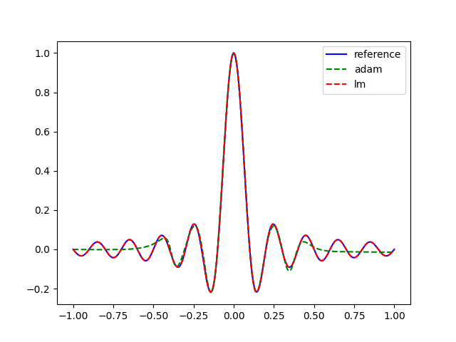
Simple curve fitting test implemented in test_curve_fitting.py and Colab. The function y = sinc(10 * x) is fitted using a Shallow Neural Network with 61 parameters.
Despite the triviality of the problem, first-order methods such as Adam fail to converge, while Levenberg-Marquardt converges rapidly with very low loss values. The values of learning_rate were chosen experimentally on the basis of the results obtained by each algorithm.
Here the results with Adam for 10000 epochs and learning_rate=0.01
Train using Adam
Epoch 1/10000
20/20 [==============================] - 0s 500us/step - loss: 0.0479
...
Epoch 10000/10000
20/20 [==============================] - 0s 449us/step - loss: 6.5928e-04
Elapsed time:  157.10102080000001
Here the results with Levenberg-Marquardt for 100 epochs and learning_rate=1.0
Train using Levenberg-Marquardt
Epoch 1/100
20/20 [==============================] - 0s 6ms/step - damping_factor: 1.0000e-05 - attempts: 2.0000 - loss: 0.0232
...
Epoch 100/100
20/20 [==============================] - 0s 5ms/step - damping_factor: 1.0000e-07 - attempts: 1.0000 - loss: 1.0265e-08
Elapsed time:  14.7972407
Plot results
Results on mnist dataset classification
Common mnist classification test implemented in test_mnist_classification.py and Colab. The classification is performed using a Convolutional Neural Network with 1026 parameters.
This time there were no particular benefits as in the previous case. Even if Levenberg-Marquardt converges with far fewer epochs than Adam, the longer execution time per step nullifies its advantages.
However, both methods achieve roughly the same accuracy values on train and test set.
Here the results with Adam for 300 epochs and learning_rate=0.01
Train using Adam
Epoch 1/200
10/10 [==============================] - 0s 28ms/step - loss: 2.0728 - accuracy: 0.3072
...
Epoch 200/200
10/10 [==============================] - 0s 14ms/step - loss: 0.0737 - accuracy: 0.9782
Elapsed time:  58.071762045000014

test_loss: 0.072342 - test_accuracy: 0.977100
Here the results with Levenberg-Marquardt for 10 epochs and learning_rate=0.1
Train using Levenberg-Marquardt
Epoch 1/10
10/10 [==============================] - 4s 434ms/step - damping_factor: 1.0000e-06 - attempts: 3.0000 - loss: 1.1267 - accuracy: 0.5803
...
Epoch 10/10
10/10 [==============================] - 5s 450ms/step - damping_factor: 1.0000e-05 - attempts: 2.0000 - loss: 0.0683 - accuracy: 0.9777
Elapsed time:  54.859995966999975

test_loss: 0.072407 - test_accuracy: 0.977800
Requirements
- Tensorflow 2.18.0
- Matplotlib to visualize curve fitting results


Download files
Download the file for your platform. If you're not sure which to choose, learn more about installing packages.
Source Distribution
Built Distribution
Filter files by name, interpreter, ABI, and platform.
If you're not sure about the file name format, learn more about wheel file names.
Copy a direct link to the current filters
File details
Details for the file tf_levenberg_marquardt-1.0.0.tar.gz.
File metadata
- Download URL: tf_levenberg_marquardt-1.0.0.tar.gz
- Upload date:
- Size: 17.3 kB
- Tags: Source
- Uploaded using Trusted Publishing? No
- Uploaded via: twine/6.0.1 CPython/3.10.15
File hashes
| Algorithm | Hash digest | |
|---|---|---|
| SHA256 |
6d42c669cf8ef32d290c98075f22be99d3df4769fc9cc22149fc2f08b70ba3ed
|
|
| MD5 |
ce9b0a4bcf3cf44f36bb807af20a63ab
|
|
| BLAKE2b-256 |
d154767992930a0bc1f1ebf6e8d6b1460f6036b2d68a890e9b5f9dd856226a06
|
File details
Details for the file tf_levenberg_marquardt-1.0.0-py3-none-any.whl.
File metadata
- Download URL: tf_levenberg_marquardt-1.0.0-py3-none-any.whl
- Upload date:
- Size: 15.4 kB
- Tags: Python 3
- Uploaded using Trusted Publishing? No
- Uploaded via: twine/6.0.1 CPython/3.10.15
File hashes
| Algorithm | Hash digest | |
|---|---|---|
| SHA256 |
91be61505079a976fde805b0e8456574db0effb2a5f35aeb4858885f5d89cd4d
|
|
| MD5 |
2d093511408376dde196594012499a5d
|
|
| BLAKE2b-256 |
7a25d7ae9609888d2f383b5de59e107a02ced0728b38ad27324d989b97742256
|


