




Introduction
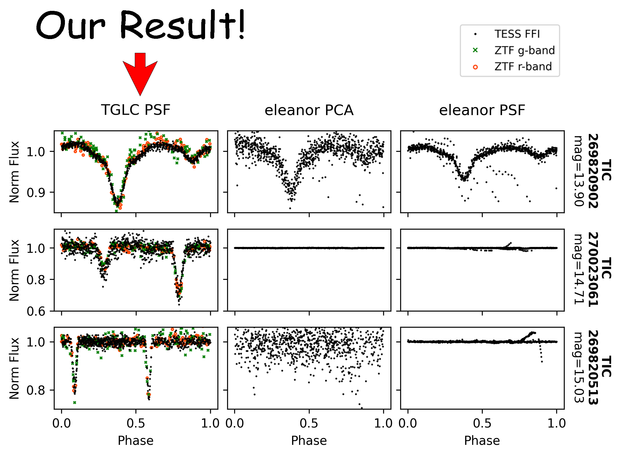
TESS-Gaia Light Curve (TGLC) is a dataset of TESS full-frame image light curves publicly available via the MAST portal. It is fitted with effective PSF and decontaminated with Gaia DR3 and achieved percent-level photometric precision down to 16th TESS magnitude! It unlocks astrophysics to a vast number of dim stars below 12th TESS magnitude. A package called tglc is pip-installable for customized light curve fits.
Usage
Historical products contain four main flux columns. TGLC 0.8.0 also writes aperture_flux_raw and psf_flux_raw, giving six flux columns. Check the product’s processing version and available columns before choosing:
aperture_flux_raw is the decontaminated 3 by 3 pixel sum; psf_flux_raw is the fitted target amplitude. Both retain signed values in electrons/second before catalog-based additive offsets and detrending. They are extracted photometry, not unprocessed detector measurements.
aperture_flux and psf_flux are not detrended, but do include catalog-based additive offsets. Aperture flux also includes the modeled aperture-fraction correction. The headers record the exact relationships: aperture_flux = (aperture_flux_raw - LOC_BG) / PORTION and psf_flux = psf_flux_raw - PSF_BG.
cal_aper_flux and cal_psf_flux are normalized and detrended. They are useful for an initial inspection of short-period signals; the default one-day detrending can alter longer stellar variations.
Compare aperture and PSF results for your target. Transit depths and stellar amplitudes depend on contamination, catalog flux estimates and the modeled aperture fraction; neither flux choice guarantees the correct amplitude. For custom calibration or detrending, start from the raw columns, inspect the offsets and quality flags, and account for remaining contamination. tglc_lc(save_aper=True) also saves the decontaminated 5 by 5 pixel cube for inspecting other apertures, whose flux fractions need their own calibration.
The tutorial shows the syntaxes and differences among these light curves in several examples.
Data Access
There are three data access methods:
MAST Portal: Easiest for acquiring light curves for a few stars. However, new sectors are updated relatively slowly.
MAST bulk download: Best for downloading light curves for all stars (<16 TESS magnitude) in a sectors.
tglc package: Generate customized light curves from available SPOC cutouts; see the workflow and limitations below.
MAST Portal/bulk download
The easiest usage requires no package installation. Simply follow the TGLC HLSP page to download light curves from MAST or use MAST Portal. Light curves are being fitted sector by sector and will be available on MAST gradually. MAST hosts all Gaia DR3 stars down to 16th magnitude. Each .fits file includes PSF and aperture light curves and their calibrated versions.
MAST available sectors: sector worklist
tglc package
Users can also fit light curves using the package tglc. Using tglc, one can specify a region, sector(s), and customized aperture shape if needed. It can also allow all field stars to float by assigning Gaussian priors, which can help decontaminate variable field stars. The supported Python range is 3.10–3.12. Use a separate environment from the MIT QLP implementation because both packages install as tglc. Run:
pip install tglc
for the latest published release. This documentation describes 0.8.0; see GitHub Releases for published versions. To install this checkout, run python -m pip install -e . from the repository directory. The 0.8.0 release notes describe changes, migration, and validation status; the 1.0 roadmap covers later work.
Important for upgrades: earlier public versions contained an error in the subpixel coordinate mapping used for bilinear interpolation. Version 0.8.0 fixes it in both ePSF fitting and target rendering. Fitted ePSFs from 0.8.0 and earlier versions are not interchangeable in either direction. Refit from the science images and rerun extraction; renaming or converting old ePSF caches is insufficient. Existing light curves remain readable but are not corrected by installation.
A single-target example:
from pathlib import Path
from tglc.quick_lc import tglc_lc, plot_lc

output = Path("tglc-output")
paths = tglc_lc(
    target=16005254,                 # equivalent to "TIC 16005254"
    local_directory=output,
    first_sector_only=True,          # choose one sector for a first run
    ffi="SPOC",
    saturation_limit=80000.0,         # conservative cutoff in electrons/second
    saturation_dilation=1,
)
print(paths)                         # FITS paths generated during this call
plot_lc(local_directory=output, ffi="SPOC")
This example contacts MAST and Gaia and downloads science data. New files are written below lc/SPOC/ (or lc/TICA/). Old files in lc/ remain separate. Path objects and strings work without a trailing slash. The saturation cutoff masks pixels during fitting; it does not establish validated photometry for saturated targets. See the usage reference and tutorial for interpreting the outputs.
Development
From a checkout, install into a dedicated virtual environment:
python -m pip install -e '.[dev]'
python -m pytest
python -m build
python -m twine check dist/*
The default test suite is offline. Network tests are marked separately. The CI workflow is configured to build and test the installed wheel on Linux and macOS with Python 3.10–3.12. The standalone scripts/quick_lc_smoketest.py downloads all available sectors and should be run deliberately, with sufficient disk space and time.
Known Problems
Catalog-based offsets and aperture fractions can change fractional amplitudes. The raw columns and reconstruction headers let users inspect these adjustments; catalog-normalized flux is not independently calibrated absolute photometry.
The configurable saturation mask protects PSF fits. Its default 80000 e-/s cutoff and one-pixel dilation are approximate, and long bleed trails can extend beyond the mask. Accurate photometry of saturated targets is not established.
TICA remains experimental. The recommended public workflow uses SPOC inputs. For precise timing, verify the target-versus-cutout reference correction; SPOC timestamps are retained without a second full barycentric correction.
Installing 0.8.0 does not regenerate existing MAST products. Check their version, flags and flux definitions separately from newly extracted files.
Reference
If you find the TGLC light curves or the tglc package useful in your research, please cite our paper published on the Astronomical Journal.
1 maintainer

Metadata
1 maintainer
Release files for tglc 0.8.0
For a detailed explanation of source distributions (sdists) and built distributions (wheels), please see the package formats documentation.
Source distribution (sdist)
| File | Size | Uploaded | |
|---|---|---|---|
| tglc-0.8.0.tar.gz | 5.3 MB | Details |
Built distribution (wheel)
| File | Interpreter | ABI | Platform | Reset |
|---|---|---|---|---|
| tglc-0.8.0-py3-none-any.whl | Python 3 | none | any | Details |
Total release size: 10.5 MB
Release files / tglc-0.8.0.tar.gz
| Download URL | tglc-0.8.0.tar.gz |
|---|---|
| Size | 5.3 MB |
| Tags | Source |
|
SHA-256 checksum How to use checksums |
f8517e374726f0edff183e2a1f71dac685c9d116e137a77d259888c7e8a4160d
|
|
BLAKE2b-256 checksum How to use checksums |
a76b9a10bb2e4188a4f527147648b1fba51333257af74e2a15445c044035dcf4
|
| Upload date | |
|
Uploaded using Trusted Publishing? What is trusted publishing? |
No |
| Uploaded via |
twine/7.0.0 CPython/3.12.14
|
Release files / tglc-0.8.0-py3-none-any.whl
| Download URL | tglc-0.8.0-py3-none-any.whl |
|---|---|
| Size | 5.3 MB |
| Tags | Python 3 |
|
SHA-256 checksum How to use checksums |
a0b73e53583c744819c8bba32d3ddf46b5ad46d2908bb7684ebe2b0f1aed494f
|
|
BLAKE2b-256 checksum How to use checksums |
c89c68adabe6af6fa9270c41c130a129f59ef61aa5f176de481fb4ac3885995e
|
| Upload date | |
|
Uploaded using Trusted Publishing? What is trusted publishing? |
No |
| Uploaded via |
twine/7.0.0 CPython/3.12.14
|














