A package for imputing missing data in time series and forecasting in missing-data contexts

Project description


timefiller is a Python package designed for time series imputation and forecasting. When applied to a set of correlated time series, each series is processed individually, utilizing both its own auto-regressive patterns and correlations with the other series. The package is user-friendly, making it accessible even to non-experts.
Originally developed for imputation, it also proves useful for forecasting, particularly when covariates contain missing values.
Why this package?
This package is an excellent choice for tasks involving missing data. It is lightweight and offers a straightforward, user-friendly API. Since its initial release, numerous enhancements have been made to accelerate data imputation, with further improvements planned for the future.
This package is ideal if:
- You have a collection of correlated time series with missing data and need to impute the missing values in one, several, or all of them
- You need to perform forecasting in scenarios with missing data, especially when dealing with unpredictable or irregular patterns, and require an algorithm capable of handling them dynamically
Installation
You can get timefiller from PyPi:
pip install timefiller
But also from conda-forge:
conda install -c conda-forge timefiller
mamba install timefiller
TimeSeriesImputer
The core of timefiller is the TimeSeriesImputer class is designed for the imputation of multivariate time series data. It extends the capabilities of ImputeMultiVariate by accounting for autoregressive and multivariate lags, as well as preprocessing.
Key Features
- Autoregressive Lags: The imputer can handle autoregressive lags, which are specified using the
ar_lagsparameter. This allows the model to use past values of the series to predict missing values. - Multivariate Lags: The imputer can also handle multivariate lags, specified using the
multivariate_lagsparameter. This allows the model to use lagged values of other series to predict missing values. - Preprocessing: The imputer supports preprocessing steps, such as scaling or normalization, which can be specified using the
preprocessingparameter. This ensures that the data is properly prepared before imputation. - Custom Estimators: The imputer can use any scikit-learn compatible estimator for the imputation process. This allows for flexibility in choosing the best model for the data.
- Handling Missing Values: The imputer can handle missing values in both the target series and the covariates. It uses the
optimasklibrary to create NaN-free train and predict matrices for the estimator. - Uncertainty Estimation: If the
alphaparameter is specified, the imputer can provide uncertainty estimates for the imputed values, by wrapping the chosen estimator with MAPIE.
Basic Usage
The simplest usage example:
from timefiller import TimeSeriesImputer

df = load_your_dataset()
tsi = TimeSeriesImputer()
df_imputed = tsi(X=df)
Advanced Usage
from sklearn.linear_model import Lasso
from timefiller import PositiveOutput, TimeSeriesImputer

df = load_your_dataset()
tsi = TimeSeriesImputer(estimator=Lasso(positive=True),
                        ar_lags=(1, 2, 3, 6, 24),
                        multivariate_lags=48,
                        negative_ar=True,
                        preprocessing=PositiveOutput())
df_imputed = tsi(X=df,
                 subset_cols=['col_1', 'col_17'],
                 after='2024-06-14',
                 n_nearest_features=75)
Check out the documentation for details on available options to customize your imputation.
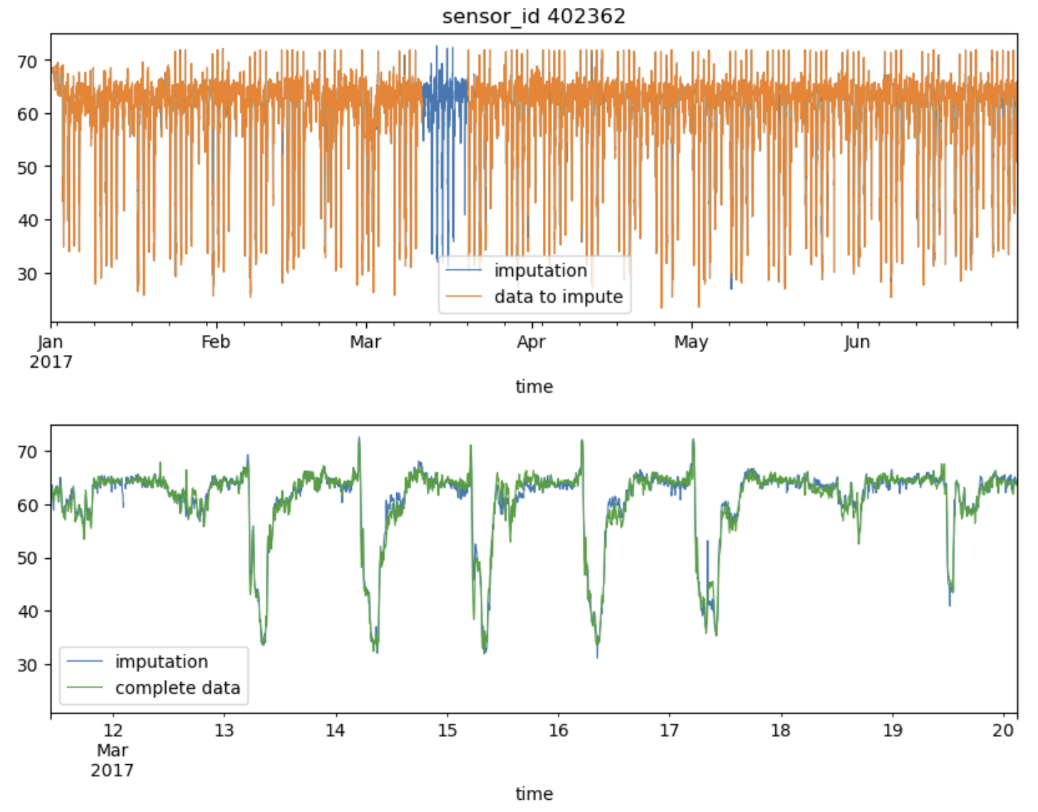
Real data example
Let's evaluate how timefiller performs on a real-world dataset, the PeMS-Bay traffic data. A sensor ID is selected for the experiment, and a contiguous block of missing values is introduced. To increase the complexity, additional Missing At Random (MAR) data is simulated, representing 1% of the entire dataset:
import matplotlib.pyplot as plt
import numpy as np
import pandas as pd
from timefiller import PositiveOutput, TimeSeriesImputer
from timefiller.utils import add_mar_nan, fetch_pems_bay

# Fetch the time series dataset (e.g., PeMS-Bay traffic data)
df = fetch_pems_bay()
df.shape, df.index.freq
>>> ((52128, 325), <5 * Minutes>)
dfm = df.copy()  # Create a copy to introduce missing values later

# Randomly select one column (sensor ID) to introduce missing values
k = np.random.randint(df.shape[1])
col = df.columns[k]
i, j = 20_000, 22_500  # Define a range in the dataset to set as NaN (missing values)
dfm.iloc[i:j, k] = np.nan  # Introduce missing values in this range for the selected column

# Add more missing values randomly across the dataset (1% of the data)
dfm = add_mar_nan(dfm, ratio=0.01)

# Initialize the TimeSeriesImputer with AR lags and multivariate lags
tsi = TimeSeriesImputer(ar_lags=(1, 2, 3, 4, 5, 10, 15, 25, 50), preprocessing=PositiveOutput())

# Apply the imputation method on the modified dataframe
%time df_imputed = tsi(dfm, subset_cols=col)
>>> CPU times: total: 7.91 s
>>> Wall time: 2.93 s
# Plot the imputed data alongside the data with missing values
df_imputed[col].rename('imputation').plot(figsize=(10, 3), lw=0.8, c='C0')
dfm[col].rename('data to impute').plot(ax=plt.gca(), lw=0.8, c='C1')
plt.title(f'sensor_id {col}')
plt.legend()
plt.show()

# Plot the imputed data vs the original complete data for comparison
df_imputed[col].rename('imputation').plot(figsize=(10, 3), lw=0.8, c='C0')
df[col].rename('complete data').plot(ax=plt.gca(), lw=0.8, c='C2')
plt.xlim(dfm.index[i], dfm.index[j])  # Focus on the region where data was missing
plt.legend()
plt.show()
Algorithmic Approach
timefiller relies heavily on scikit-learn for the learning process and uses optimask to create NaN-free train and
predict matrices for the estimator.
For each column requiring imputation, the algorithm differentiates between rows with valid data and those with missing values. For rows with missing data, it identifies the available sets of other columns (features). For each set, OptiMask is called to train the chosen sklearn estimator on the largest possible submatrix without any NaNs. This process can become computationally expensive if the available sets of features vary greatly or occur infrequently. In such cases, multiple calls to OptiMask and repeated fitting and predicting using the estimator may be necessary.
One important point to keep in mind is that within a single column, two different rows (timestamps) may be imputed using different estimators (regressors), each trained on distinct sets of columns (covariate features) and samples (rows/timestamps).
Release history Release notifications | RSS feed


Download files
Download the file for your platform. If you're not sure which to choose, learn more about installing packages.
Source Distribution
Built Distribution
Filter files by name, interpreter, ABI, and platform.
If you're not sure about the file name format, learn more about wheel file names.
Copy a direct link to the current filters
File details
Details for the file timefiller-1.0.6.tar.gz.
File metadata
- Download URL: timefiller-1.0.6.tar.gz
- Upload date:
- Size: 23.3 kB
- Tags: Source
- Uploaded using Trusted Publishing? No
- Uploaded via: twine/6.0.1 CPython/3.12.8
File hashes
| Algorithm | Hash digest | |
|---|---|---|
| SHA256 |
23d74fb6a8927732a74b0122cc70f617ea4a3d5a98f56e10e82d83e92fb48520
|
|
| MD5 |
8e28ea5abdf9f229b8de8ca3f6b46f68
|
|
| BLAKE2b-256 |
1b10caa248e12dee1fc0793bc7bc247e2b4e5e3d869e4ebb2bd63e3c39da08e7
|
File details
Details for the file timefiller-1.0.6-py3-none-any.whl.
File metadata
- Download URL: timefiller-1.0.6-py3-none-any.whl
- Upload date:
- Size: 20.6 kB
- Tags: Python 3
- Uploaded using Trusted Publishing? No
- Uploaded via: twine/6.0.1 CPython/3.12.8
File hashes
| Algorithm | Hash digest | |
|---|---|---|
| SHA256 |
98c74630dc180c184d5feb8c03a376cf52af383b73311582f2bb36dc35f6ba07
|
|
| MD5 |
7dd3d2d2b8d88151d7922d0081d29218
|
|
| BLAKE2b-256 |
1b45ef412406dbc5978f6bc3197c51a9ec304089a83141a00026a1b7dabbb950
|


