Transition Network Analysis for Python

Project description
TNA - Transition Network Analysis for Python
A Python package providing exact numerical equivalence to the R TNA package for analyzing sequential data as transition networks.
Features
- 8 Model Types: relative, frequency, co-occurrence, reverse, n-gram, gap, window, attention
- 9 Centrality Measures: OutStrength, InStrength, ClosenessIn, ClosenessOut, Closeness, Betweenness, BetweennessRSP, Diffusion, Clustering
- Statistical Inference: Bootstrap resampling, permutation tests, confidence intervals
- 10+ Visualization Functions: Network plots, heatmaps, centrality charts, sequence plots
- R Package Equivalence: Verified numerical equivalence with comprehensive test suite
Installation
# Latest stable version
pip install tnapy

# Development installation
pip install -e .

# Or install dependencies directly
pip install numpy pandas networkx scipy matplotlib seaborn
Quick Start
import tna
import pandas as pd
# Load example data (2000 learning sessions with 9 self-regulated learning behaviors)
df = tna.load_group_regulation()
# Build a TNA model (relative transition probabilities)
model = tna.tna(df)
print(model)
# Compute centrality measures
cent = tna.centralities(model)
print(cent)
# Visualize the network
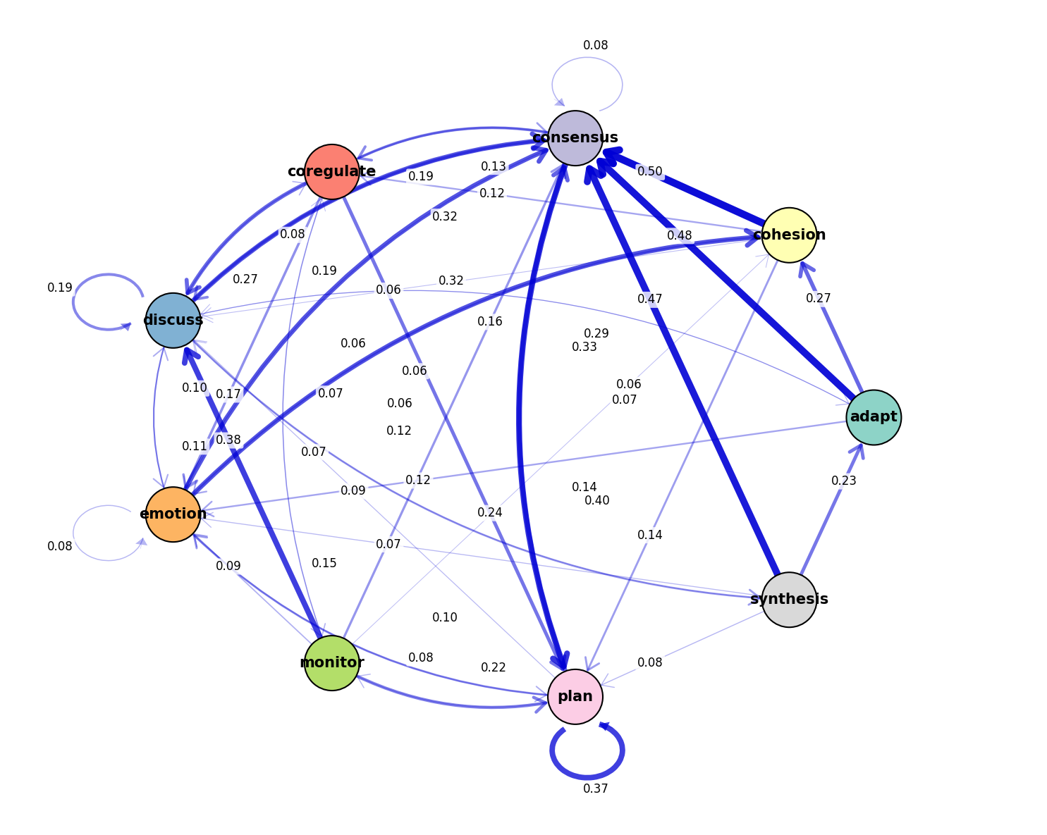
tna.plot_network(model, layout='circular', edge_threshold=0.05)
# Visualize centralities
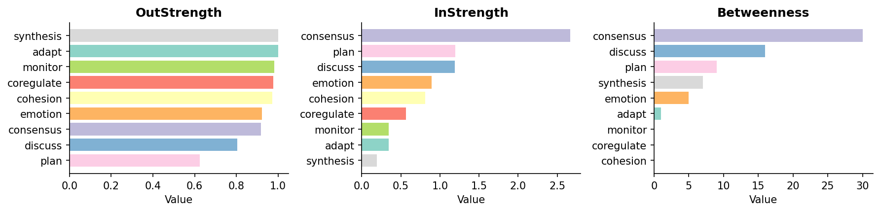
tna.plot_centralities(cent, measures=['OutStrength', 'InStrength', 'Betweenness'])
Output:
TNA Model
  Type: relative
  States: ['adapt', 'cohesion', 'consensus', 'coregulate', 'discuss', 'emotion', 'monitor', 'plan', 'synthesis']
  Scaling: none

Transition Matrix:
               adapt  cohesion  consensus  coregulate   discuss   emotion   monitor      plan  synthesis
adapt       0.000000  0.273084   0.477407    0.021611  0.058939  0.119843  0.033399  0.015717   0.000000
cohesion    0.002950  0.027139   0.497935    0.119174  0.059587  0.115634  0.033038  0.141003   0.003540
consensus   0.004740  0.014852   0.082003    0.187707  0.188023  0.072681  0.046611  0.395797   0.007584
coregulate  0.016244  0.036041   0.134518    0.023350  0.273604  0.172081  0.086294  0.239086   0.018782
discuss     0.071374  0.047583   0.321185    0.084282  0.194887  0.105796  0.022273  0.011643   0.140977
emotion     0.002467  0.325344   0.320409    0.034191  0.101868  0.076842  0.036306  0.099753   0.002820
monitor     0.011165  0.055827   0.159107    0.057920  0.375436  0.090719  0.018144  0.215632   0.016050
plan        0.000975  0.025175   0.290401    0.017216  0.067890  0.146825  0.075524  0.374208   0.001787
synthesis   0.234663  0.033742   0.466258    0.044479  0.062883  0.070552  0.012270  0.075153   0.000000

Centralities:
            OutStrength  InStrength  ClosenessIn  ClosenessOut  Closeness  Betweenness  BetweennessRSP  Diffusion  Clustering
adapt          1.000000    0.344578     0.131494      0.142857   0.142857          0.0        0.029498   5.586292    0.336984
cohesion       0.972861    0.811648     0.137931      0.142857   0.142857          0.0        0.072174   5.208633    0.299649
consensus      0.917997    2.667219     0.142857      0.137931   0.142857          0.0        0.082498   4.659728    0.160777
coregulate     0.976650    0.566581     0.133333      0.142857   0.142857          0.0        0.062987   5.147938    0.305784
discuss        0.805113    1.188232     0.138889      0.138889   0.142857          0.0        0.089174   4.627577    0.239711
emotion        0.923158    0.894131     0.136986      0.142857   0.142857          0.0        0.070595   5.069888    0.290479
monitor        0.981856    0.345715     0.131868      0.142857   0.142857          0.0        0.044498   5.156837    0.288882
plan           0.625792    1.193784     0.142857      0.133333   0.142857          0.0        0.094078   3.487529    0.287490
synthesis      1.000000    0.191539     0.126984      0.142857   0.142857          0.0        0.024055   5.582502    0.358614
Network Plot:
Centralities Plot:
Model Building
Basic Models
# Relative transition probabilities (default)
model = tna.tna(df)

# Frequency model (raw counts)
fmodel = tna.ftna(df)

# Co-occurrence model (bidirectional)
cmodel = tna.ctna(df)

# Attention model (exponential decay weighting)
amodel = tna.atna(df, beta=0.1)
Advanced Model Types
# All model types via build_model()
model = tna.build_model(df, type_='relative')      # Row-normalized probabilities
model = tna.build_model(df, type_='frequency')     # Raw transition counts
model = tna.build_model(df, type_='co-occurrence') # Bidirectional co-occurrence
model = tna.build_model(df, type_='reverse')       # Reverse order transitions
model = tna.build_model(df, type_='n-gram', params={'n': 2})  # Higher-order n-grams
model = tna.build_model(df, type_='gap', params={'max_gap': 3, 'decay': 0.5})  # Gap-weighted
model = tna.build_model(df, type_='window', params={'size': 3})  # Sliding window
model = tna.build_model(df, type_='attention', params={'beta': 0.1})  # Attention-weighted
Scaling Options
# Apply scaling to weight matrix
model = tna.tna(df, scaling='minmax')  # Min-max normalization [0, 1]
model = tna.tna(df, scaling='max')     # Divide by maximum
model = tna.tna(df, scaling='rank')    # Rank-based scaling
model = tna.tna(df, scaling=['minmax', 'max'])  # Multiple scalings
Centrality Measures
# Compute all centrality measures
cent = tna.centralities(model)

# Compute specific measures
cent = tna.centralities(model, measures=['OutStrength', 'InStrength', 'Betweenness'])

# With normalization
cent = tna.centralities(model, normalize=True)

# Include self-loops
cent = tna.centralities(model, loops=True)
Available Measures
| Measure | Description |
|---|---|
OutStrength |
Sum of outgoing edge weights |
InStrength |
Sum of incoming edge weights |
ClosenessIn |
Incoming closeness centrality |
ClosenessOut |
Outgoing closeness centrality |
Closeness |
Overall closeness (treats graph as undirected) |
Betweenness |
Standard betweenness centrality |
BetweennessRSP |
Randomized Shortest Path betweenness |
Diffusion |
Diffusion centrality (Banerjee et al. 2014) |
Clustering |
Weighted clustering coefficient (Zhang & Horvath 2005) |
Data Preparation
From Long Format Data
# Prepare raw event data
prepared = tna.prepare_data(
    data=events_df,
    actor='user_id',
    time='timestamp',
    action='event_type',
    time_threshold=900  # 15 minutes session timeout
)

# Build model from prepared data
model = tna.tna(prepared)

# Access statistics
print(prepared.statistics)  # n_sessions, n_actors, etc.
From Wide Format Data
# Direct from wide format (rows=sequences, cols=time steps)
df = pd.DataFrame({
    'step1': ['A', 'B', 'A'],
    'step2': ['B', 'C', 'C'],
    'step3': ['C', 'A', 'B']
})
model = tna.tna(df)
Statistical Inference
Bootstrap Analysis
# Bootstrap confidence intervals for model parameters
boot = tna.bootstrap_tna(df, n_boot=1000, ci=0.95, seed=42)

# Get summary with CIs for all edges
summary = boot.summary()

# Find significant edges
sig_edges = boot.significant_edges(threshold=0)

# Bootstrap centrality measures
cent_ci = tna.bootstrap_centralities(
    df,
    measures=['OutStrength', 'InStrength', 'Betweenness'],
    n_boot=1000,
    ci=0.95
)
Permutation Tests
# Compare two groups
result = tna.permutation_test(
    group1_df, group2_df,
    n_perm=1000,
    statistic='weights',  # or 'density', 'centrality'
    alternative='two-sided',
    seed=42
)
print(f"P-value: {result.p_value}")
print(f"Significant: {result.is_significant(0.05)}")

# Edge-wise comparison with multiple testing correction
edges = tna.permutation_test_edges(
    group1_df, group2_df,
    n_perm=1000,
    correction='fdr'  # or 'bonferroni', 'none'
)
Confidence Intervals
# Percentile method
ci = tna.confidence_interval(boot_samples, ci=0.95, method='percentile')

# BCa method (bias-corrected and accelerated)
ci = tna.bca_ci(data, boot_samples, statistic_func=np.mean, ci=0.95)
Visualization
Network Plots
# Basic network plot
tna.plot_network(model)

# Customized network
tna.plot_network(
    model,
    layout='circular',           # or 'spring', 'kamada_kawai'
    node_size='OutStrength',     # Size by centrality
    edge_threshold=0.05,         # Hide weak edges
    node_color='steelblue',
    edge_cmap='Blues'
)

# Network with bootstrap confidence intervals
tna.plot_network_ci(boot, edge_alpha='significance')
Centrality Plots
# Bar charts for centralities
tna.plot_centralities(
    cent,
    measures=['OutStrength', 'InStrength', 'Betweenness'],
    ncol=3
)
Heatmap
# Transition matrix heatmap
tna.plot_heatmap(model, cmap='Blues', annotate=True)
Model Comparison
# Side-by-side comparison of two models
tna.plot_comparison(
    model1, model2,
    plot_type='heatmap',
    labels=('Group 1', 'Group 2')
)
Sequence Visualization
# State distribution over time
tna.plot_sequences(df, plot_type='distribution')

# State frequencies
tna.plot_frequencies(df)

# Histogram of sequence lengths
tna.plot_histogram(df)
Statistical Plots
# Bootstrap distribution
tna.plot_bootstrap(boot, plot_type='weights')
tna.plot_bootstrap(boot, plot_type='centrality', measure='OutStrength')

# Permutation test null distribution
tna.plot_permutation(result)
Example Datasets
# Wide format: 2000 sessions x 20 time steps
df = tna.load_group_regulation()

# Long format: Actor, Time, Action columns
df_long = tna.load_group_regulation_long()
API Reference
Model Building
| Function | Description |
|---|---|
tna(x) |
Build relative transition probability model |
ftna(x) |
Build frequency (raw counts) model |
ctna(x) |
Build co-occurrence model |
atna(x, beta) |
Build attention-weighted model |
build_model(x, type_) |
Build model with specified type |
Data Preparation
| Function | Description |
|---|---|
prepare_data(data, actor, time, action) |
Prepare long-format event data |
create_seqdata(x) |
Create sequence data from various formats |
Centralities
| Function | Description |
|---|---|
centralities(model, measures) |
Compute centrality measures |
Statistical Inference
| Function | Description |
|---|---|
bootstrap_tna(x, n_boot) |
Bootstrap analysis of TNA model |
bootstrap_centralities(x, measures, n_boot) |
Bootstrap centrality CIs |
permutation_test(x1, x2, n_perm) |
Permutation test for group comparison |
permutation_test_edges(x1, x2, n_perm) |
Edge-wise permutation tests |
confidence_interval(samples, ci) |
Calculate confidence interval |
bca_ci(data, samples, func, ci) |
BCa confidence interval |
Visualization
| Function | Description |
|---|---|
plot_network(model) |
Plot transition network |
plot_centralities(cent) |
Plot centrality bar charts |
plot_heatmap(model) |
Plot transition matrix heatmap |
plot_comparison(m1, m2) |
Compare two models |
plot_sequences(df) |
Plot sequence patterns |
plot_frequencies(df) |
Plot state frequencies |
plot_histogram(df) |
Plot sequence length histogram |
plot_bootstrap(boot) |
Visualize bootstrap results |
plot_permutation(result) |
Visualize permutation test |
plot_network_ci(boot) |
Network with confidence intervals |
Utilities
| Function | Description |
|---|---|
row_normalize(matrix) |
Row-normalize a matrix |
minmax_scale(matrix) |
Min-max scaling to [0, 1] |
max_scale(matrix) |
Divide by maximum |
rank_scale(matrix) |
Rank-based scaling |
R Package Equivalence
This package is designed to produce numerically equivalent results to the R TNA package. Key equivalences:
- Transition matrices: Identical computation of relative, frequency, and co-occurrence matrices
- Centrality measures: Exact ports of R implementations including custom measures (diffusion, weighted clustering)
- Data format: Compatible with R's wide-format sequence data
Verification
# Python
model_py = tna.tna(df)
cent_py = tna.centralities(model_py)

# Results match R within floating-point precision:
# - Max absolute difference < 1e-10 for transition matrices
# - Max absolute difference < 1e-6 for centrality measures
Citation
If you use this package in your research, please cite:
@software{tna_python,
  title = {TNA: Transition Network Analysis for Python},
  author  = "Saqr, Mohammed and Tikka, Santtu and López-Pernas, Sonsoles",
  year = {2026},
  url = {https://github.com/mohsaqr/tnapy}
}
Also cite Transition Network Analysis as a method
@INPROCEEDINGS{Saqr2025-ku,
  title     = "Transition Network Analysis: A Novel Framework for Modeling,
               Visualizing, and Identifying the Temporal Patterns of Learners
               and Learning Processes",
  author    = "Saqr, Mohammed and López-Pernas, Sonsoles and Törmänen, Tiina and
               Kaliisa, Rogers and Misiejuk, Kamila and Tikka, Santtu",
  booktitle = "Proceedings of Learning Analytics \& Knowledge (LAK '25)",
  publisher = "ACM",
  address   = "New York, NY, USA",
  doi       = "10.1145/3706468.3706513",
  pages     = "351 - 361",
  year      =  2025
}
License
MIT License
Contributing
Contributions are welcome! Please feel free to submit a Pull Request.
Release history Release notifications | RSS feed


Download files
Download the file for your platform. If you're not sure which to choose, learn more about installing packages.
Source Distribution
Built Distribution
Filter files by name, interpreter, ABI, and platform.
If you're not sure about the file name format, learn more about wheel file names.
Copy a direct link to the current filters
File details
Details for the file tnapy-0.2.0.tar.gz.
File metadata
- Download URL: tnapy-0.2.0.tar.gz
- Upload date:
- Size: 170.7 kB
- Tags: Source
- Uploaded using Trusted Publishing? No
- Uploaded via: twine/6.2.0 CPython/3.9.6
File hashes
| Algorithm | Hash digest | |
|---|---|---|
| SHA256 |
8a75ff59684e1946182788de881300e4a7e38e643afc97582d68626b8ddbe527
|
|
| MD5 |
6d13e4e9d27ef328dc45572e0246c93b
|
|
| BLAKE2b-256 |
8ac545579d85446e471120a8fba97b904580c602598abdc2a3f39d2a85edc5fe
|
File details
Details for the file tnapy-0.2.0-py3-none-any.whl.
File metadata
- Download URL: tnapy-0.2.0-py3-none-any.whl
- Upload date:
- Size: 140.7 kB
- Tags: Python 3
- Uploaded using Trusted Publishing? No
- Uploaded via: twine/6.2.0 CPython/3.9.6
File hashes
| Algorithm | Hash digest | |
|---|---|---|
| SHA256 |
2df7849ffa53597bc29f4c70d76e4d6ee32474cb170109109a8ea997d11615b5
|
|
| MD5 |
b3a8f083a452a6fa08bd5baac4619d1c
|
|
| BLAKE2b-256 |
20ad922451c0be3dcc57fb9ae80e07f9e399248d4cf1c924d0db56b6e76f37bf
|


