Pandas implementation of institutional-grade multi-factor risk model (Polars original by 0xfdf/toraniko)

Project description
toraniko-pandas 
Pandas implementation of institutional-grade multi-factor risk model (Polars original by 0xfdf/toraniko)
Changelog
New Statistical Functions
The following functions in extras.py are inspired by the techniques described in "The Elements of Quantitative Investing" by Giuseppe A. Paleologo:
-
Covariance Estimation
shrinkage_cov: Implementation of Ledoit & Wolf's optimal shrinkage method for covariance matricesewma_cov: Exponentially Weighted Moving Average for covariance estimationlagged_covs: Calculation of lag-based covariance matrices for time series data
-
Autocorrelation-Consistent Covariance Estimation
autocorr_cov: Autocorrelation-consistent estimator for factor covariancenwest_cov: Newey-West estimator for heteroskedasticity and autocorrelation consistent covariance
-
CVXPY Optimization
estimate_factor_returns_cvxpy: Constrained optimization for factor return estimation_factor_returns_cvxpy: Implementation of the convex optimization approach with sum-zero constraints
These functions provide robust statistical methods for portfolio management, risk modeling, and factor analysis as described in modern quantitative finance literature.
Installation
pip install toraniko_pandas
User Manual
This notebook demonstrates factor analysis using SimFin financial data and custom factor models.
Important
You need free API key from SimFin to run my example. See their Github for more info. Create a .env file and place it like below
# SimFin
SIMFIN_API_KEY = "YOUR_KEY"
Data
import warnings

import matplotlib.pyplot as plt
import statsmodels.api as sm

from simfin_downloader import SimFin
from toraniko_pandas.model import estimate_factor_returns
from toraniko_pandas.styles import factor_mom, factor_sze, factor_val
from toraniko_pandas.utils import top_n_by_group

# Configure warnings
warnings.simplefilter(action="ignore", category=FutureWarning)
warnings.filterwarnings("ignore", message="invalid value encountered in log")
warnings.filterwarnings("ignore", message="divide by zero encountered in log")
simfin = SimFin()
df, sectors, industries = simfin.get_toraniko_data()

# Filter top 3000 companies by market cap
df = top_n_by_group(df.dropna(), 3000, "market_cap", ("date",), True)
# Display sector data
sectors
| sector_basic_materials | sector_business_services | sector_consumer_cyclical | sector_consumer_defensive | sector_energy | sector_financial_services | sector_healthcare | sector_industrials | sector_other | sector_real_estate | sector_technology | sector_utilities | |
|---|---|---|---|---|---|---|---|---|---|---|---|---|
| symbol | ||||||||||||
| A | 0 | 0 | 0 | 0 | 0 | 0 | 1 | 0 | 0 | 0 | 0 | 0 |
| AA | 1 | 0 | 0 | 0 | 0 | 0 | 0 | 0 | 0 | 0 | 0 | 0 |
| AAC | 0 | 0 | 0 | 0 | 0 | 1 | 0 | 0 | 0 | 0 | 0 | 0 |
| AACI | 0 | 0 | 0 | 0 | 0 | 1 | 0 | 0 | 0 | 0 | 0 | 0 |
| AAC_delisted | 0 | 0 | 0 | 0 | 0 | 0 | 1 | 0 | 0 | 0 | 0 | 0 |
| ... | ... | ... | ... | ... | ... | ... | ... | ... | ... | ... | ... | ... |
| ZWS | 0 | 0 | 0 | 0 | 0 | 0 | 0 | 1 | 0 | 0 | 0 | 0 |
| ZY | 0 | 0 | 0 | 0 | 0 | 0 | 1 | 0 | 0 | 0 | 0 | 0 |
| ZYME | 0 | 0 | 0 | 0 | 0 | 0 | 1 | 0 | 0 | 0 | 0 | 0 |
| ZYNE | 0 | 0 | 0 | 0 | 0 | 0 | 1 | 0 | 0 | 0 | 0 | 0 |
| ZYXI | 0 | 0 | 0 | 0 | 0 | 0 | 1 | 0 | 0 | 0 | 0 | 0 |
5766 rows × 12 columns
# Display industry data
industries
| industry_advertising_and_marketing_services | industry_aerospace_and_defense | industry_agriculture | industry_airlines | industry_alternative_energy_sources_and_other | industry_application_software | industry_asset_management | industry_autos | industry_banks | industry_beverages_-_alcoholic | ... | industry_retail_-_defensive | industry_semiconductors | industry_steel | industry_tobacco_products | industry_transportation_and_logistics | industry_travel_and_leisure | industry_truck_manufacturing | industry_utilities_-_independent_power_producers | industry_utilities_-_regulated | industry_waste_management | |
|---|---|---|---|---|---|---|---|---|---|---|---|---|---|---|---|---|---|---|---|---|---|
| symbol | |||||||||||||||||||||
| A | 0 | 0 | 0 | 0 | 0 | 0 | 0 | 0 | 0 | 0 | ... | 0 | 0 | 0 | 0 | 0 | 0 | 0 | 0 | 0 | 0 |
| AA | 0 | 0 | 0 | 0 | 0 | 0 | 0 | 0 | 0 | 0 | ... | 0 | 0 | 0 | 0 | 0 | 0 | 0 | 0 | 0 | 0 |
| AAC | 0 | 0 | 0 | 0 | 0 | 0 | 0 | 0 | 1 | 0 | ... | 0 | 0 | 0 | 0 | 0 | 0 | 0 | 0 | 0 | 0 |
| AACI | 0 | 0 | 0 | 0 | 0 | 0 | 0 | 0 | 1 | 0 | ... | 0 | 0 | 0 | 0 | 0 | 0 | 0 | 0 | 0 | 0 |
| AAC_delisted | 0 | 0 | 0 | 0 | 0 | 0 | 0 | 0 | 0 | 0 | ... | 0 | 0 | 0 | 0 | 0 | 0 | 0 | 0 | 0 | 0 |
| ... | ... | ... | ... | ... | ... | ... | ... | ... | ... | ... | ... | ... | ... | ... | ... | ... | ... | ... | ... | ... | |
| ZWS | 0 | 0 | 0 | 0 | 0 | 0 | 0 | 0 | 0 | 0 | ... | 0 | 0 | 0 | 0 | 0 | 0 | 0 | 0 | 0 | 0 |
| ZY | 0 | 0 | 0 | 0 | 0 | 0 | 0 | 0 | 0 | 0 | ... | 0 | 0 | 0 | 0 | 0 | 0 | 0 | 0 | 0 | 0 |
| ZYME | 0 | 0 | 0 | 0 | 0 | 0 | 0 | 0 | 0 | 0 | ... | 0 | 0 | 0 | 0 | 0 | 0 | 0 | 0 | 0 | 0 |
| ZYNE | 0 | 0 | 0 | 0 | 0 | 0 | 0 | 0 | 0 | 0 | ... | 0 | 0 | 0 | 0 | 0 | 0 | 0 | 0 | 0 | 0 |
| ZYXI | 0 | 0 | 0 | 0 | 0 | 0 | 0 | 0 | 0 | 0 | ... | 0 | 0 | 0 | 0 | 0 | 0 | 0 | 0 | 0 | 0 |
5766 rows × 74 columns
# Asset returns was calculated by taking the percentage change of the adjusted close prices
ret_df = df[["symbol", "asset_returns"]]
ret_df
| symbol | asset_returns | |
|---|---|---|
| date | ||
| 2019-04-01 | EOSS | 0.041667 |
| 2019-04-01 | YTEN | 0.017544 |
| 2019-04-01 | GIDYL | 0.000000 |
| 2019-04-01 | VISL | -0.028571 |
| 2019-04-01 | ASLE | -0.001020 |
| ... | ... | ... |
| 2024-02-16 | NLY | -0.012099 |
| 2024-02-16 | AAPL | -0.008461 |
| 2024-02-16 | MSFT | -0.006159 |
| 2024-02-16 | WPC | 0.001669 |
| 2024-02-16 | RENT | -0.045675 |
3406422 rows × 2 columns
# Market cap is used to calculate the size factor and later to select the top N by market cap
cap_df = df[["symbol", "market_cap"]]
cap_df
| symbol | market_cap | |
|---|---|---|
| date | ||
| 2019-04-01 | EOSS | 1.600000e+05 |
| 2019-04-01 | YTEN | 2.939904e+05 |
| 2019-04-01 | GIDYL | 3.113633e+05 |
| 2019-04-01 | VISL | 3.423120e+05 |
| 2019-04-01 | ASLE | 3.623279e+05 |
| ... | ... | ... |
| 2024-02-16 | NLY | 2.291316e+12 |
| 2024-02-16 | AAPL | 2.865508e+12 |
| 2024-02-16 | MSFT | 3.016308e+12 |
| 2024-02-16 | WPC | 3.098176e+12 |
| 2024-02-16 | RENT | 8.506228e+12 |
3406422 rows × 2 columns
# To calculate the sector scores, we merge the sectors dataframe with the main dataframe
sector_scores = (
    df.reset_index()
    .merge(sectors, on="symbol")
    .set_index("date")[["symbol"] + sectors.columns.tolist()]
)
sector_scores
| symbol | sector_basic_materials | sector_business_services | sector_consumer_cyclical | sector_consumer_defensive | sector_energy | sector_financial_services | sector_healthcare | sector_industrials | sector_other | sector_real_estate | sector_technology | sector_utilities | |
|---|---|---|---|---|---|---|---|---|---|---|---|---|---|
| date | |||||||||||||
| 2019-04-01 | EOSS | 0 | 0 | 0 | 1 | 0 | 0 | 0 | 0 | 0 | 0 | 0 | 0 |
| 2019-04-01 | YTEN | 1 | 0 | 0 | 0 | 0 | 0 | 0 | 0 | 0 | 0 | 0 | 0 |
| 2019-04-01 | VISL | 0 | 0 | 0 | 0 | 0 | 0 | 0 | 0 | 0 | 0 | 1 | 0 |
| 2019-04-01 | ASLE | 0 | 0 | 0 | 0 | 0 | 0 | 0 | 1 | 0 | 0 | 0 | 0 |
| 2019-04-01 | ALBO | 0 | 0 | 0 | 0 | 0 | 0 | 1 | 0 | 0 | 0 | 0 | 0 |
| ... | ... | ... | ... | ... | ... | ... | ... | ... | ... | ... | ... | ... | ... |
| 2024-02-16 | NLY | 0 | 0 | 0 | 0 | 0 | 1 | 0 | 0 | 0 | 0 | 0 | 0 |
| 2024-02-16 | AAPL | 0 | 0 | 0 | 0 | 0 | 0 | 0 | 0 | 0 | 0 | 1 | 0 |
| 2024-02-16 | MSFT | 0 | 0 | 0 | 0 | 0 | 0 | 0 | 0 | 0 | 0 | 1 | 0 |
| 2024-02-16 | WPC | 0 | 0 | 0 | 0 | 0 | 0 | 0 | 0 | 0 | 1 | 0 | 0 |
| 2024-02-16 | RENT | 0 | 0 | 1 | 0 | 0 | 0 | 0 | 0 | 0 | 0 | 0 | 0 |
3393141 rows × 13 columns
# Size factor calculation
size_df = factor_sze(df, lower_decile=0.2, upper_decile=0.8)

# Momentum factor calculation
mom_df = factor_mom(df, trailing_days=252, winsor_factor=0.01)

# Value factor calculation
value_df = factor_val(df, winsor_factor=0.05)
# Momentum distribution
mom_df["mom_score"].hist(bins=100)
plt.title("Momentum Factor Distribution")
plt.show()

# Value distribution
value_df["val_score"].hist(bins=100)
plt.title("Value Factor Distribution")
plt.show()


# %%  All of which we merge to get the style scores
style_scores = (
    value_df.merge(mom_df, on=["symbol", "date"])
    .merge(size_df, on=["symbol", "date"])
    .dropna()
)
style_scores
| symbol | val_score | mom_score | sze_score | |
|---|---|---|---|---|
| date | ||||
| 2020-04-28 | ALBO | 2.732799 | -0.308748 | 3.418444 |
| 2020-04-28 | HSDT | 2.441402 | -1.777434 | 3.316239 |
| 2020-04-28 | ASLE | 1.547939 | 0.836804 | 3.259800 |
| 2020-04-28 | VISL | 2.732799 | -1.571045 | 3.042578 |
| 2020-04-28 | KNWN | 1.570320 | -0.325302 | 2.970678 |
| ... | ... | ... | ... | ... |
| 2024-02-16 | NLY | -2.076270 | 0.015212 | -2.906904 |
| 2024-02-16 | AAPL | -1.156765 | 0.344759 | -2.996094 |
| 2024-02-16 | MSFT | -0.963887 | 0.876672 | -3.016549 |
| 2024-02-16 | WPC | -2.877029 | -0.090848 | -3.027231 |
| 2024-02-16 | RENT | -2.327684 | -2.079591 | -3.430058 |
2479098 rows × 4 columns
ddf = (
    ret_df.merge(cap_df, on=["date", "symbol"])
    .merge(sector_scores, on=["date", "symbol"])
    .merge(style_scores, on=["date", "symbol"])
    .dropna()
    .astype({"symbol": "category"})
)
returns_df = ddf[["symbol", "asset_returns"]]
mkt_cap_df = ddf[["symbol", "market_cap"]]
sector_df = ddf[["symbol"] + sectors.columns.tolist()]
style_df = ddf[style_scores.columns]
fac_df, eps_df = estimate_factor_returns(
    returns_df,
    mkt_cap_df,
    sector_df,
    style_df,
    winsor_factor=0.1,
    residualize_styles=False,
)
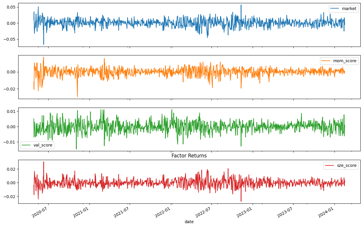
factor_cols = ["market","mom_score", "val_score", "sze_score"]

fac_df[factor_cols].plot(subplots=True, figsize=(15, 10))
plt.title("Factor Returns")
plt.show()

(fac_df[factor_cols] + 1).cumprod().plot(figsize=(15, 10))
plt.title("Factor Returns Cumulative")
plt.show()

y = returns_df.query("symbol == 'AAPL'")["asset_returns"]
X = fac_df[["market", "sector_technology", "mom_score", "val_score", "sze_score"]]
X = sm.add_constant(X)

model = sm.OLS(y, X)
results = model.fit().get_robustcov_results()
results.summary()
| Dep. Variable: | asset_returns | R-squared: | 0.610 |
|---|---|---|---|
| Model: | OLS | Adj. R-squared: | 0.608 |
| Method: | Least Squares | F-statistic: | 259.8 |
| Date: | Fri, 21 Feb 2025 | Prob (F-statistic): | 3.77e-175 |
| Time: | 10:42:32 | Log-Likelihood: | 2914.3 |
| No. Observations: | 959 | AIC: | -5817. |
| Df Residuals: | 953 | BIC: | -5787. |
| Df Model: | 5 | ||
| Covariance Type: | HC1 |
| coef | std err | t | P>|t| | [0.025 | 0.975] | |
|---|---|---|---|---|---|---|
| const | 0.0004 | 0.000 | 0.955 | 0.340 | -0.000 | 0.001 |
| market | -1.3258 | 0.175 | -7.594 | 0.000 | -1.668 | -0.983 |
| sector_technology | 0.3238 | 0.087 | 3.738 | 0.000 | 0.154 | 0.494 |
| mom_score | 0.4925 | 0.095 | 5.211 | 0.000 | 0.307 | 0.678 |
| val_score | -1.4278 | 0.233 | -6.140 | 0.000 | -1.884 | -0.971 |
| sze_score | -4.6804 | 0.389 | -12.030 | 0.000 | -5.444 | -3.917 |
| Omnibus: | 241.840 | Durbin-Watson: | 1.897 |
|---|---|---|---|
| Prob(Omnibus): | 0.000 | Jarque-Bera (JB): | 2493.520 |
| Skew: | 0.841 | Prob(JB): | 0.00 |
| Kurtosis: | 10.718 | Cond. No. | 1.14e+03 |
Notes:
[1] Standard Errors are heteroscedasticity robust (HC1)
[2] The condition number is large, 1.14e+03. This might indicate that there are
strong multicollinearity or other numerical problems.
The strong multicollinearity is due to the estimated market factor derived from the sectors is almost correlated 1:1 with the sze factor.
Release history Release notifications | RSS feed


Download files
Download the file for your platform. If you're not sure which to choose, learn more about installing packages.
Source Distribution
Built Distribution
Filter files by name, interpreter, ABI, and platform.
If you're not sure about the file name format, learn more about wheel file names.
Copy a direct link to the current filters
File details
Details for the file toraniko_pandas-0.1.2.tar.gz.
File metadata
- Download URL: toraniko_pandas-0.1.2.tar.gz
- Upload date:
- Size: 139.9 kB
- Tags: Source
- Uploaded using Trusted Publishing? No
- Uploaded via: uv/0.6.7
File hashes
| Algorithm | Hash digest | |
|---|---|---|
| SHA256 |
d8f54be008d6cd45f39451bc54c9fe631fc07ecdf3c41507f8c63dc2a167ca08
|
|
| MD5 |
1909d3fcbda206e21562a7579c3bf207
|
|
| BLAKE2b-256 |
2bc43390770a9390a83ba36c0fe201ad0290158bc26a5e9aa9781ebf73e536af
|
File details
Details for the file toraniko_pandas-0.1.2-py3-none-any.whl.
File metadata
- Download URL: toraniko_pandas-0.1.2-py3-none-any.whl
- Upload date:
- Size: 18.1 kB
- Tags: Python 3
- Uploaded using Trusted Publishing? No
- Uploaded via: uv/0.6.7
File hashes
| Algorithm | Hash digest | |
|---|---|---|
| SHA256 |
98fdf86f8fd5d6b4618ea46ea36d94e18bffa780d2b7466a34718c7eec859e1a
|
|
| MD5 |
2fc7cb0bdf5ffb2fe4aa6318979dc076
|
|
| BLAKE2b-256 |
beea7cb2d533ae6d52fb6ac97798a6a5bf8822e187a4c6474fcfd94b7f2dc1c9
|


