Building blocks for Continual Inference Networks in PyTorch

Project description

A Python library for Continual Inference Networks in PyTorch
Quick-start • Docs • Principles • Paper • Examples • Modules • Model Zoo • Contribute • License
Continual Inference Networks ensure efficient stream processing
Many of our favorite Deep Neural Network architectures (e.g., CNNs and Transformers) were built with offline-processing for offline processing. Rather than processing inputs one sequence element at a time, they require the whole (spatio-)temporal sequence to be passed as a single input. Yet, many important real-life applications need online predictions on a continual input stream. While CNNs and Transformers can be applied by re-assembling and passing sequences within a sliding window, this is inefficient due to the redundant intermediary computations from overlapping clips.
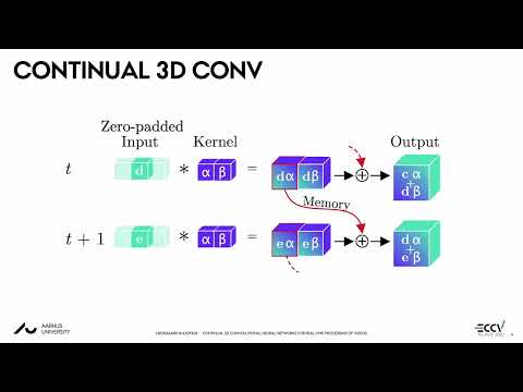
Continual Inference Networks (CINs) ensure efficient stream processing via an alternative computational ordering, with ~L × fewer FLOPs per prediction compared to sliding window-based inference with non-CINs where L is the corresponding sequence length of a non-CIN network. For details on their inner workings, check out the videos below or the corresponding papers [1, 2].
News
- 2022-12-02: ONNX compatibility for all modules is available from v1.0.0. See test_onnx.py for examples.
Quick-start
Install
pip install continual-inference
Example
co modules are weight-compatible drop-in replacement for torch.nn, enhanced with the capability of efficient continual inference:
import torch
import continual as co

#                      B, C, T, H, W
example = torch.randn((1, 1, 5, 3, 3))

conv = co.Conv3d(in_channels=1, out_channels=1, kernel_size=(3, 3, 3))

# Same exact computation as torch.nn.Conv3d ✅
output = conv(example)

# But can also perform online inference efficiently 🚀
firsts = conv.forward_steps(example[:, :, :4])
last = conv.forward_step(example[:, :, 4])

assert torch.allclose(output[:, :, : conv.delay], firsts)
assert torch.allclose(output[:, :, conv.delay], last)

# Temporal properties
assert conv.receptive_field == 3
assert conv.delay == 2
See the network composition and model zoo sections for additional examples.
Library principles
Forward modes
The library components feature three distinct forward modes, which are handy for different situations, namely forward, forward_step, and forward_steps:
forward(input)
Performs a forward computation over multiple time-steps. This function is identical to the corresponding module in torch.nn, ensuring cross-compatibility. Moreover, it's handy for efficient training on clip-based data.
         O            (O: output)
         ↑
         N            (N: network module)
         ↑
 -----------------    (-: aggregation)
 P   I   I   I   P    (I: input frame, P: padding)
forward_step(input, update_state=True)
Performs a forward computation for a single frame and (optionally) updates internal states accordingly. This function performs efficient continual inference.
O+S O+S O+S O+S   (O: output, S: updated internal state)
 ↑   ↑   ↑   ↑
 N   N   N   N    (N: network module)
 ↑   ↑   ↑   ↑
 I   I   I   I    (I: input frame)
forward_steps(input, pad_end=False, update_state=True)
Performs a forward computation across multiple time-steps while updating internal states for continual inference (if update_state=True). Start-padding is always accounted for, but end-padding is omitted per default in expectance of the next input step. It can be added by specifying pad_end=True. If so, the output-input mapping the exact same as that of forward.
         O            (O: output)
         ↑
 -----------------    (-: aggregation)
 O  O+S O+S O+S  O    (O: output, S: updated internal state)
 ↑   ↑   ↑   ↑   ↑
 N   N   N   N   N    (N: network module)
 ↑   ↑   ↑   ↑   ↑
 P   I   I   I   P    (I: input frame, P: padding)
__call__
Per default, the __call__ function operates identically to torch.nn and executes forward. We supply two options for changing this behavior, namely the call_mode property and the call_mode context manager. An example of their use follows:
timeseries = torch.randn(batch, channel, time)
timestep = timeseries[:, :, 0]

net(timeseries)  # Invokes net.forward(timeseries)

# Assign permanent call_mode property
net.call_mode = "forward_step"
net(timestep)  # Invokes net.forward_step(timestep)

# Assign temporary call_mode with context manager
with co.call_mode("forward_steps"):
    net(timeseries)  # Invokes net.forward_steps(timeseries)

net(timestep)  # Invokes net.forward_step(timestep) again
Composition
Continual Inference Networks require strict handling of internal data delays to guarantee correspondence between forward modes. While it is possible to compose neural networks by defining forward, forward_step, and forward_steps manually, correct handling of delays is cumbersome and time-consuming. Instead, we provide a rich interface of container modules, which handles delays automatically. On top of co.Sequential (which is a drop-in replacement of torch.nn.Sequential), we provide modules for handling parallel and conditional dataflow.
co.Sequential: Invoke modules sequentially, passing the output of one module onto the next.co.Broadcast: Broadcast one stream to multiple.co.Parallel: Invoke modules in parallel given each their input.co.ParallelDispatch: Dispatch multiple input streams to multiple output streams flexibly.co.Reduce: Reduce multiple input streams to one.co.BroadcastReduce: Shorthand for Sequential(Broadcast, Parallel, Reduce).co.Residual: Residual connection.co.Conditional: Conditionally checks whether to invoke a module (or another) at runtime.
Composition examples:
Residual module
Short-hand:
residual = co.Residual(co.Conv3d(32, 32, kernel_size=3, padding=1))
Explicit:
residual = co.Sequential(
    co.Broadcast(2),
    co.Parallel(
        co.Conv3d(32, 32, kernel_size=3, padding=1),
        co.Delay(2),
    ),
    co.Reduce("sum"),
)
3D MobileNetV2 Inverted residual block
Continual 3D version of the MobileNetV2 Inverted residual block.
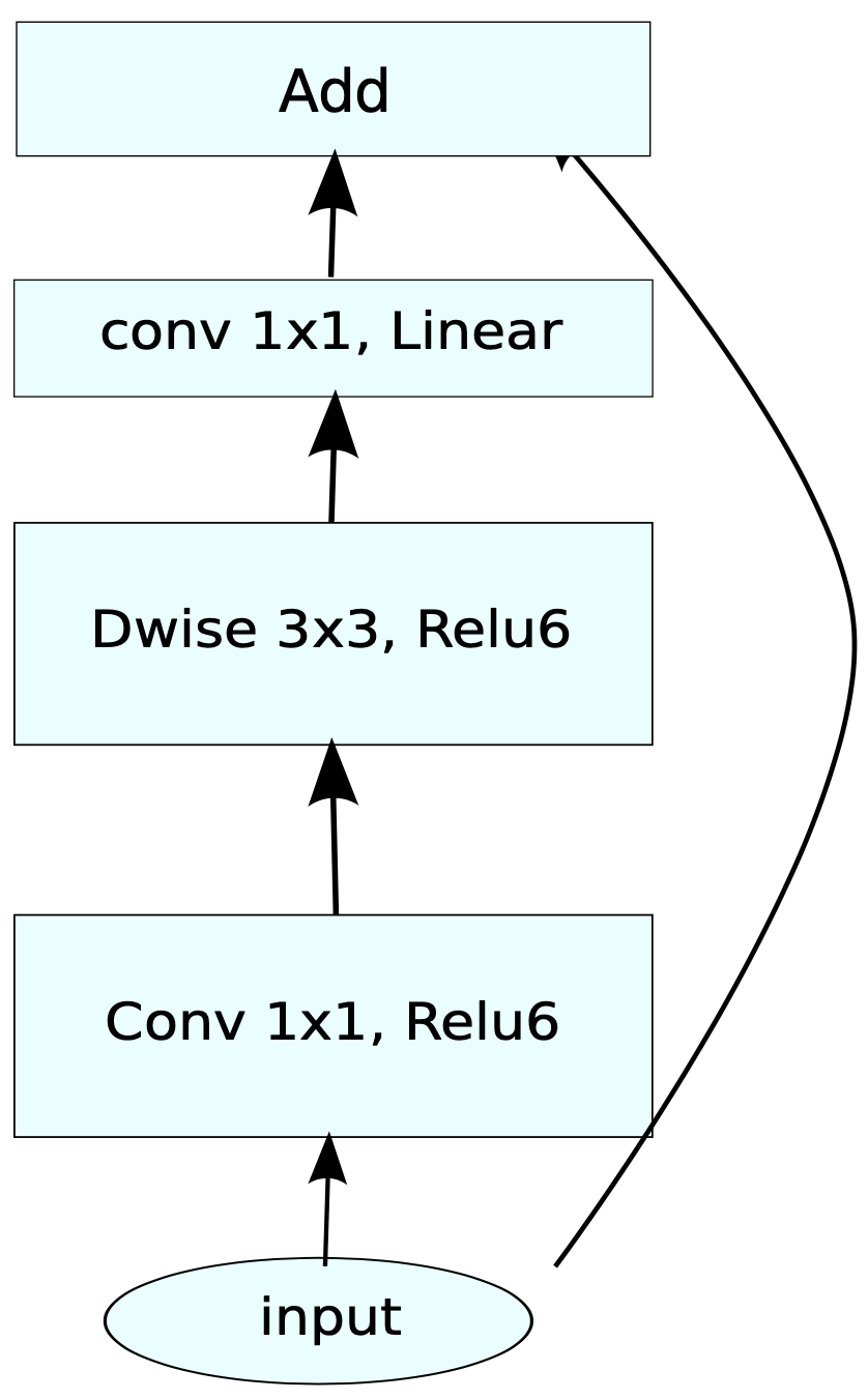
MobileNetV2 Inverted residual block. Source: https://arxiv.org/pdf/1801.04381.pdf
mb_conv = co.Residual(
    co.Sequential(
      co.Conv3d(32, 64, kernel_size=(1, 1, 1)),
      nn.BatchNorm3d(64),
      nn.ReLU6(),
      co.Conv3d(64, 64, kernel_size=(3, 3, 3), padding=(1, 1, 1), groups=64),
      nn.ReLU6(),
      co.Conv3d(64, 32, kernel_size=(1, 1, 1)),
      nn.BatchNorm3d(32),
    )
)
3D Squeeze-and-Excitation module
Continual 3D version of the Squeeze-and-Excitation module
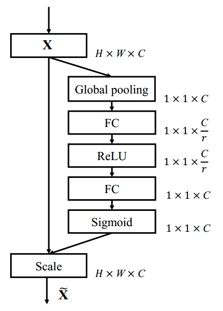
Squeeze-and-Excitation block. Scale refers to a broadcasted element-wise multiplication. Adapted from: https://arxiv.org/pdf/1709.01507.pdf
se = co.Residual(
    co.Sequential(
        OrderedDict([
            ("pool", co.AdaptiveAvgPool3d((1, 1, 1), kernel_size=7)),
            ("down", co.Conv3d(256, 16, kernel_size=1)),
            ("act1", nn.ReLU()),
            ("up", co.Conv3d(16, 256, kernel_size=1)),
            ("act2", nn.Sigmoid()),
        ])
    ),
    reduce="mul",
)
3D Inception module
Continual 3D version of the Inception module:
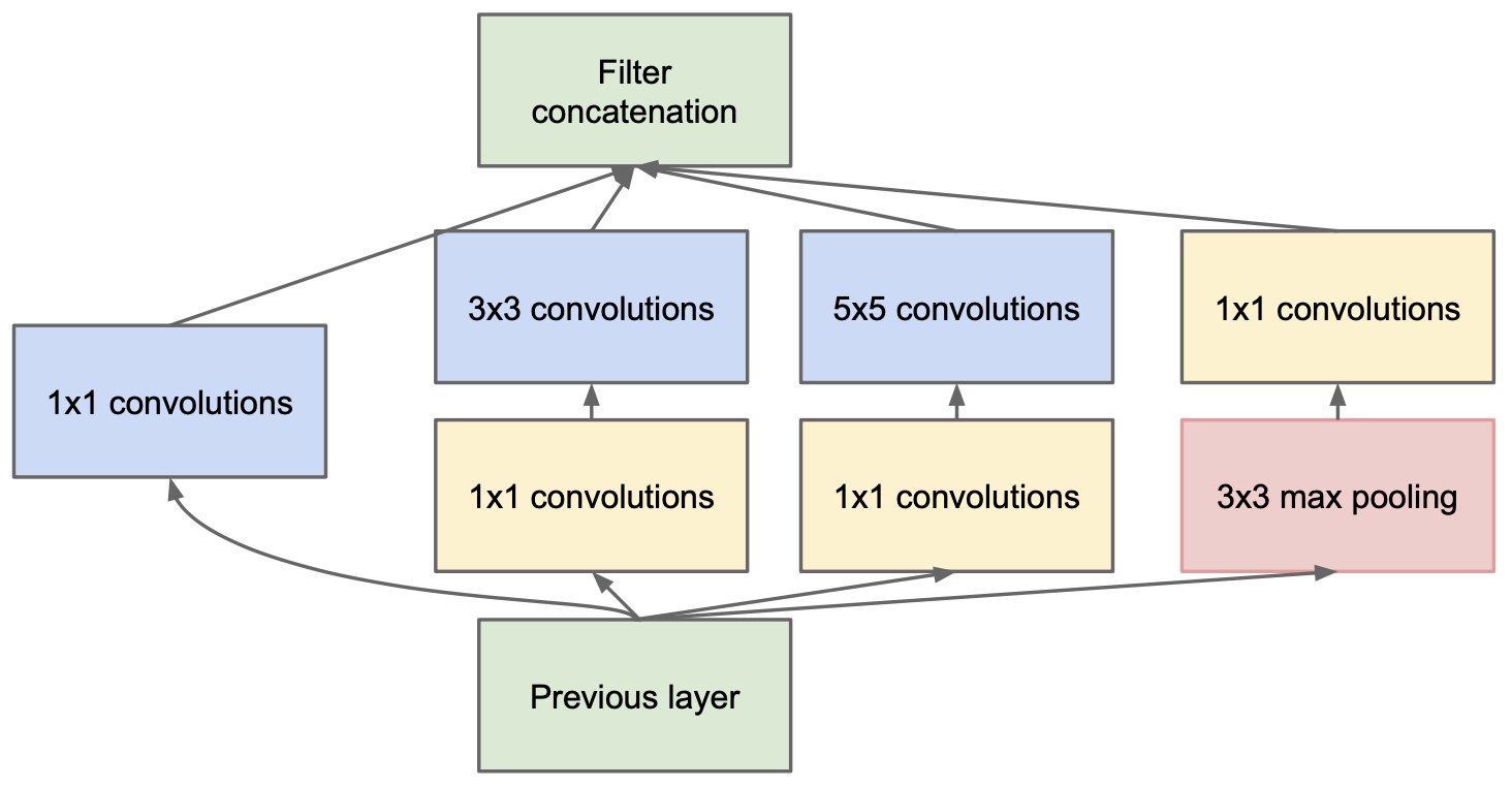
Inception module. Source: https://arxiv.org/pdf/1409.4842v1.pdf
def norm_relu(module, channels):
    return co.Sequential(
        module,
        nn.BatchNorm3d(channels),
        nn.ReLU(),
    )

inception_module = co.BroadcastReduce(
    co.Conv3d(192, 64, kernel_size=1),
    co.Sequential(
        norm_relu(co.Conv3d(192, 96, kernel_size=1), 96),
        norm_relu(co.Conv3d(96, 128, kernel_size=3, padding=1), 128),
    ),
    co.Sequential(
        norm_relu(co.Conv3d(192, 16, kernel_size=1), 16),
        norm_relu(co.Conv3d(16, 32, kernel_size=5, padding=2), 32),
    ),
    co.Sequential(
        co.MaxPool3d(kernel_size=(1, 3, 3), padding=(0, 1, 1), stride=1),
        norm_relu(co.Conv3d(192, 32, kernel_size=1), 32),
    ),
    reduce="concat",
)
Input shapes
We enforce a unified ordering of input dimensions for all library modules, namely:
(batch, channel, time, optional_dim2, optional_dim3)
Outputs
The outputs produces by forward_step and forward_steps are identical to those of forward, provided the same data was input beforehand and state update was enabled. We know that input and output shapes aren't necessarily the same when using forward in the PyTorch library, and generally depends on padding, stride and receptive field of a module.
For the forward_step function, this comes to show by some None-valued outputs. Specifically, modules with a delay (i.e. with receptive fields larger than the padding + 1) will produce None until the input count exceeds the delay. Moreover, stride > 1 will produce Tensor outputs every stride steps and None the remaining steps. A visual example is shown below:
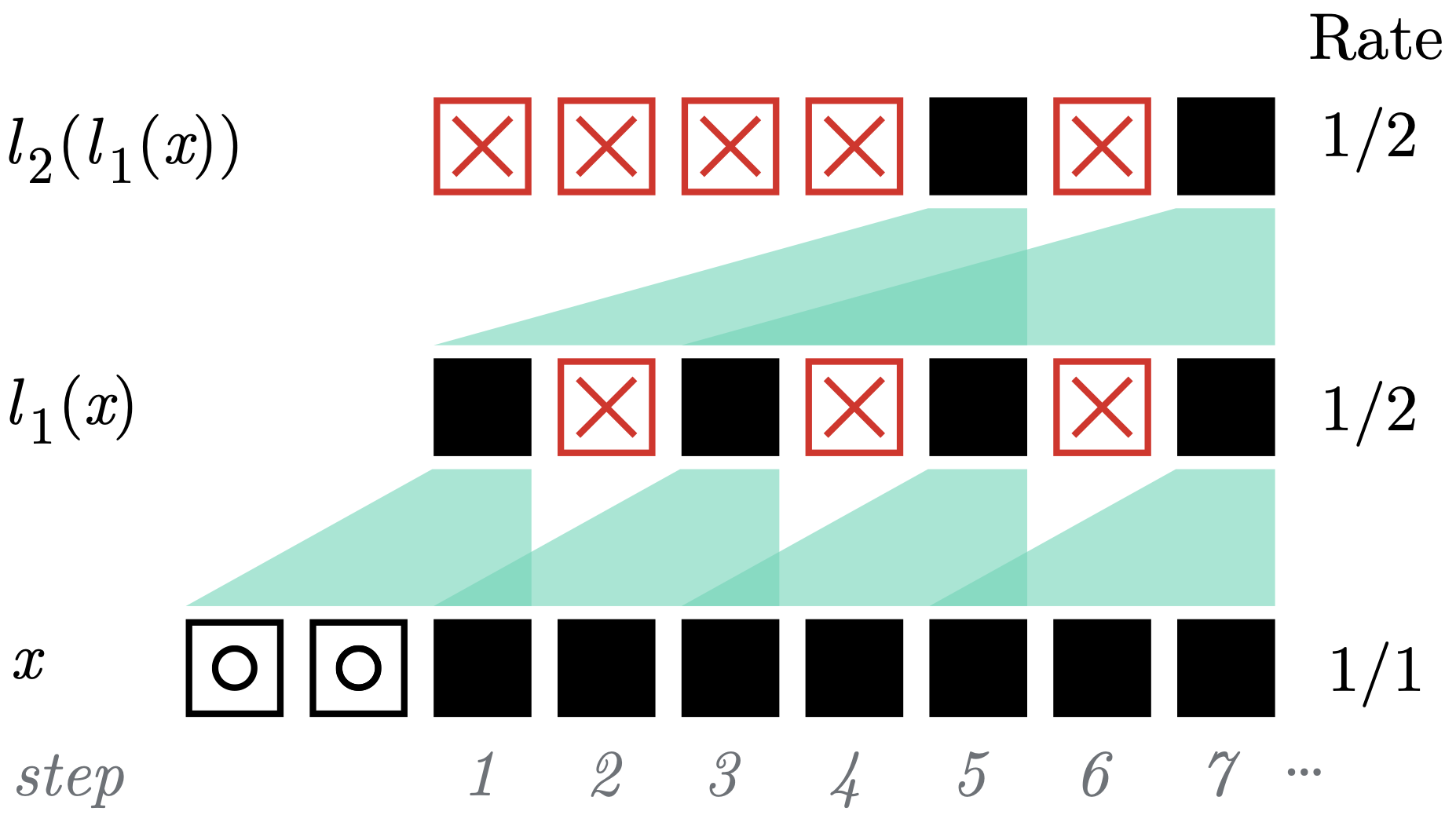
A mixed example of delay and outputs under padding and stride. Here, we illustrate the step-wise operation of two co module layers, l1 with with receptive_field = 3, padding = 2, and stride = 2 and l2 with receptive_field = 3, no padding and stride = 1. ⧇ denotes a padded zero, ■ is a non-zero step-feature, and ☒ is an empty output.
For more information, please see the library paper.
Module library
Continual Inference features a rich collection of modules for defining Continual Inference Networks. Specific care was taken to create CIN versions of the PyTorch modules found in torch.nn:
Pooling
Linear
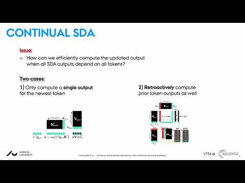
Transformers
co.TransformerEncoderco.TransformerEncoderLayerFactory: Factory function corresponding tonn.TransformerEncoderLayer.co.SingleOutputTransformerEncoderLayer: SingleOutputMHA version ofnn.TransformerEncoderLayer.co.RetroactiveTransformerEncoderLayer: RetroactiveMHA version ofnn.TransformerEncoderLayer.co.RetroactiveMultiheadAttention: Retroactive version ofnn.MultiheadAttention.co.SingleOutputMultiheadAttention: Single-output version ofnn.MultiheadAttention.co.RecyclingPositionalEncoding: Positional Encoding used for Continual Transformers.
Modules for composing and converting networks. Both composition and utility modules can be used for regular definition of PyTorch modules as well.
Composition modules
co.Sequential: Invoke modules sequentially, passing the output of one module onto the next.co.Broadcast: Broadcast one stream to multiple.co.Parallel: Invoke modules in parallel given each their input.co.ParallelDispatch: Dispatch multiple input streams to multiple output streams flexibly.co.Reduce: Reduce multiple input streams to one.co.BroadcastReduce: Shorthand for Sequential(Broadcast, Parallel, Reduce).co.Residual: Residual connection.co.Conditional: Conditionally checks whether to invoke a module (or another) at runtime.
Utility modules
co.Delay: Pure delay module (e.g. needed in residuals).co.Reshape: Reshape non-temporal dimensions.co.Lambda: Lambda module which wraps any function.co.Add: Adds a constant value.co.Multiply: Multiplies with a constant factor.co.Unity: Maps input to output without modification.co.Constant: Maps input to and output with constant value.co.Zero: Maps input to output of zeros.co.One: Maps input to output of ones.
Converters
co.continual: conversion function fromtorch.nnmodules tocomodules.co.forward_stepping: functional wrapper, which enhances temporally localtorch.nnmodules with the forward_stepping functions.
We support drop-in interoperability with with the following torch.nn modules:
Activation
nn.Thresholdnn.ReLUnn.RReLUnn.Hardtanhnn.ReLU6nn.Sigmoidnn.Hardsigmoidnn.Tanhnn.SiLUnn.Hardswishnn.ELUnn.CELUnn.SELUnn.GLUnn.GELUnn.Hardshrinknn.LeakyReLUnn.LogSigmoidnn.Softplusnn.Softshrinknn.PReLUnn.Softsignnn.Tanhshrinknn.Softminnn.Softmaxnn.Softmax2dnn.LogSoftmax
Normalization
nn.BatchNorm1dnn.BatchNorm2dnn.BatchNorm3dnn.LayerNorm
Dropout
nn.Dropoutnn.Dropout2dnn.Dropout3dnn.AlphaDropoutnn.FeatureAlphaDropout
Model Zoo and Benchmarks
Continual 3D CNNs
Benchmark results for 1-view testing on Kinetics400. For reference, X3D-L scores 69.3% top-1 acc with 19.2 GFLOPs per prediction.
| Arch | Avg. pool size | Top 1 (%) | FLOPs (G) per step | FLOPs reduction | Params (M) | Code | Weights |
|---|---|---|---|---|---|---|---|
| CoX3D-L | 64 | 71.6 | 1.25 | 15.3x | 6.2 | link | link |
| CoX3D-M | 64 | 71.0 | 0.33 | 15.1x | 3.8 | link | link |
| CoX3D-S | 64 | 64.7 | 0.17 | 12.1x | 3.8 | link | link |
| CoSlow | 64 | 73.1 | 6.90 | 8.0x | 32.5 | link | link |
| CoI3D | 64 | 64.0 | 5.68 | 5.0x | 28.0 | link | link |
FLOPs reduction is noted relative to non-continual inference. Note that on-hardware inference doesn't reach the same speedups as "FLOPs reductions" might suggest due to overhead of state reads and writes. This overhead is less important for large batch sizes. This applies to all models in the model zoo.
Continual ST-GCNs
Benchmark results for on NTU RGB+D 60 for the joint modality. For reference, ST-GCN achieves 86% X-Sub and 93.4 X-View accuracy with 16.73 GFLOPs per prediction.
| Arch | Receptive field | X-Sub Acc (%) | X-View Acc (%) | FLOPs (G) per step | FLOPs reduction | Params (M) | Code |
|---|---|---|---|---|---|---|---|
| CoST-GCN | 300 | 86.3 | 93.8 | 0.16 | 107.7x | 3.1 | link |
| CoA-GCN | 300 | 84.1 | 92.6 | 0.17 | 108.7x | 3.5 | link |
| CoST-GCN | 300 | 86.3 | 92.4 | 0.15 | 107.6x | 3.1 | link |
Here, you can download pre-trained,model weights for the above architectures on NTU RGB+D 60, NTU RGB+D 120, and Kinetics-400 on joint and bone modalities.
Continual Transformers
Benchmark results for on THUMOS14 on top of features extracted using a TSN-ResNet50 backbone pre-trained on Kinetics400. For reference, OadTR achieves 64.4 % mAP with 2.5 GFLOPs per prediction.
| Arch | Receptive field | mAP (%) | FLOPs (G) per step | Params (M) | Code |
|---|---|---|---|---|---|
| CoOadTR-b1 | 64 | 64.2 | 0.41 | 15.9 | link |
| CoOadTR-b2 | 64 | 64.4 | 0.01 | 9.6 | link |
The library features complete implementations of the one- and two-block continual transformer encoders as well.
Compatibility
The library modules are built to integrate seamlessly with other PyTorch projects. Specifically, extra care was taken to ensure out-of-the-box compatibility with:
Citation
@inproceedings{hedegaard2022colib,
  title={Continual Inference: A Library for Efficient Online Inference with Deep Neural Networks in PyTorch},
  author={Lukas Hedegaard and Alexandros Iosifidis},
  booktitle={European Conference on Computer Vision Workshops (ECCVW)},
  year={2022}
}
Acknowledgement
This work has received funding from the European Union’s Horizon 2020 research and innovation programme under grant agreement No 871449 (OpenDR).
Release history Release notifications | RSS feed

Download files
Download the file for your platform. If you're not sure which to choose, learn more about installing packages.
Source Distribution
Built Distribution
Filter files by name, interpreter, ABI, and platform.
If you're not sure about the file name format, learn more about wheel file names.
Copy a direct link to the current filters
File details
Details for the file torch-stream-0.0.1.tar.gz.
File metadata
- Download URL: torch-stream-0.0.1.tar.gz
- Upload date:
- Size: 64.9 kB
- Tags: Source
- Uploaded using Trusted Publishing? No
- Uploaded via: twine/3.4.2 importlib_metadata/4.6.3 pkginfo/1.7.1 requests/2.26.0 requests-toolbelt/0.9.1 tqdm/4.62.0 CPython/3.9.6
File hashes
| Algorithm | Hash digest | |
|---|---|---|
| SHA256 |
dff41e55a91f477c31ca9c48a6b1d06639907e25346c1cec898f2331b69fd89e
|
|
| MD5 |
39029f2da23e7c89aa0f3300c0de6e7a
|
|
| BLAKE2b-256 |
eb7ecb62463c385e3b357204c30c337f8b0dadf7e54cb7e401edd9c3a0cfdb94
|
File details
Details for the file torch_stream-0.0.1-py3-none-any.whl.
File metadata
- Download URL: torch_stream-0.0.1-py3-none-any.whl
- Upload date:
- Size: 68.4 kB
- Tags: Python 3
- Uploaded using Trusted Publishing? No
- Uploaded via: twine/3.4.2 importlib_metadata/4.6.3 pkginfo/1.7.1 requests/2.26.0 requests-toolbelt/0.9.1 tqdm/4.62.0 CPython/3.9.6
File hashes
| Algorithm | Hash digest | |
|---|---|---|
| SHA256 |
5ac36d364a46760ea298dc4f9e5fd45cd69d1d251fda94c05f0be32795a14370
|
|
| MD5 |
3f79d07bf446d904113e8f73ee309344
|
|
| BLAKE2b-256 |
ac9c121741998b17205289683801ec5729c936b43614d498389bf5917cfe0ac4
|


