PyTorch module for differentiable parametric curves with learnable coefficients
Verified details
These details have been verified by PyPIProject links
GitHub Statistics
Maintainers

Project description


A PyTorch module for vectorized and differentiable parametric curves with learnable coefficients, such as a B-spline curve with learnable control points, for KANs, continuous embeddings, and shape constraints.
Use cases
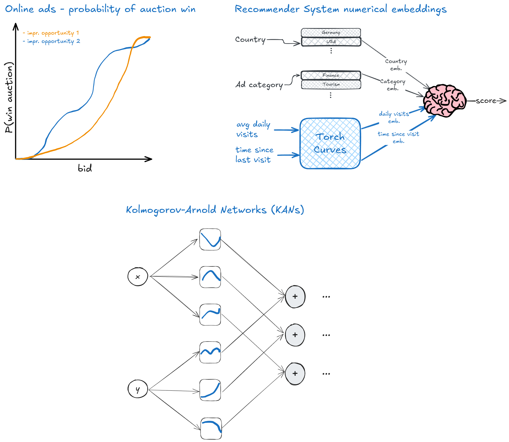
Turns out all the above use cases have one thing in common: they can all be expressed using learnable parametric curves, and that is exactly what this library provides.
Learn
A simple "hello world" example: evaluate three two-dimensional B-spline curves at four points:
import torch
import torchcurves as tc

u = torch.rand(4, 3)        # (B, C)
curve = tc.BSplineCurve(
    num_curves=3,           # C
    dim=2,                  # D
)
y = curve(u)                # (B, C, D)

print(u.shape, "->", y.shape)            # torch.Size([4, 3]) -> torch.Size([4, 3, 2])
If the coefficients come from another network instead of living inside the module,
use tc.BSplineBasis and pass the coefficients explicitly at forward time.
For more information:
- Documentation site.
- Example notebooks for you to try out.
Features
- Differentiable: Custom autograd function ensures gradients flow properly through the curve evaluation.
- Vectorized: Vectorized operations for efficient batch and multi-curve evaluation.
- Efficient numerics: Clenshaw recursion for polynomials, Cox-DeBoor for splines.
Installation
With pip:
pip install torchcurves
With uv:
uv add torchcurves
Use cases
There are examples in the doc/source/examples directory showing how to build models using
this library. Here we show some simple code snippets to appreciate the library.
Use case 1 - continuous embeddings
import torchcurves as tc
from torch import nn
import torch


class Net(nn.Module):
    def __init__(self, num_categorical, num_numerical, dim, num_knots=10):
        super().__init__()
        self.cat_emb = nn.Embedding(num_categorical, dim)
        self.num_emb = tc.BSplineCurve(num_numerical, dim, knots_config=num_knots)
        self.embedding_based_model = MySuperDuperModel()  # placeholder for your encoder model

    def forward(self, x_categorical, x_numerical):
        embeddings = torch.cat([
            self.cat_emb(x_categorical),
            self.num_emb(x_numerical)
        ], dim=-2)
        return self.embedding_based_model(embeddings)
MySuperDuperModel is a placeholder for your downstream architecture.
Use case 2 - monotone functions
Working on online advertising, and want to model the probability of winning an ad auction given the bid? We know higher bids must result in a higher win probability, so we need a monotone function. Turns out B-splines are monotone if their coefficient vectors are monotone. Want an increasing function? Ensure the spline coefficients are increasing, and the resulting spline will be monotone increasing.
Below is an example with an auction encoder that encodes the auction into a vector, we then transform it to an increasing vector, and use it as the coefficient vector for a B-spline curve.
import torch
from torch import nn
import torchcurves as tc


class AuctionWinModel(nn.Module):
    def __init__(self, num_auction_features, num_bid_coefficients):
        super().__init__()
        self.auction_encoder = make_auction_encoder(  # placeholder: an MLP, a transformer, etc.
            input_features=num_auction_features,
            output_features=num_bid_coefficients,
        )
        self.bid_basis = tc.BSplineBasis(
            degree=3,
            knots_config=num_bid_coefficients,
            input_map=tc.maps.Nonneg.rational(),
        )

    def forward(self, auction_features, bids):
        # map auction features to increasing spline coefficients
        spline_coeffs = self._make_increasing(self.auction_encoder(auction_features))

        # each mini-batch sample is treated as its own curve
        return self.bid_basis(
            bids.unsqueeze(0),           # 1 x B (B curves in 1 dimension)
            spline_coeffs.unsqueeze(-1), # B x C x 1 (B curves with C coefs in 1 dimension)
        ).squeeze(0).squeeze(-1)

    def _make_increasing(self, x):
        # transform a mini-batch of vectors to a mini-batch of increasing vectors
        initial = x[..., :1]
        increments = nn.functional.softplus(x[..., 1:])
        concatenated = torch.concat((initial, increments), dim=-1)
        return torch.cumsum(concatenated, dim=-1)
make_auction_encoder is a placeholder for your encoder architecture.
Now we can train the model to predict the probability of winning auctions given auction features and bid:
import torch.nn.functional as F

for auction_features, bids, win_labels in train_loader:
    win_logits = model(auction_features, bids)
    loss = F.binary_cross_entropy_with_logits(  # or any loss we desire
        win_logits,
        win_labels
    )

    optimizer.zero_grad()
    loss.backward()
    optimizer.step()
Use case 3 - Kolmogorov-Arnold networks
A KAN [1] based on the B-spline basis, along the lines of the original paper:
import torchcurves as tc
from torch import nn

input_dim = 2
intermediate_dim = 5
num_control_points = 10

kan = nn.Sequential(
    # layer 1
    tc.BSplineCurve(input_dim, intermediate_dim, knots_config=num_control_points),
    tc.Sum(dim=-2),
    # layer 2
    tc.BSplineCurve(intermediate_dim, intermediate_dim, knots_config=num_control_points),
    tc.Sum(dim=-2),
    # layer 3
    tc.BSplineCurve(intermediate_dim, 1, knots_config=num_control_points),
    tc.Sum(dim=-2),
)
Yes, we know the original KAN paper used a different curve parametrization, B-spline + arcsinh, but the whole point of this repo is showing that KAN activations can be parametrized in arbitrary ways.
For example, here is a KAN based on Legendre polynomials of degree 5:
import torchcurves as tc
from torch import nn

input_dim = 2
intermediate_dim = 5
degree = 5

kan = nn.Sequential(
    # layer 1
    tc.LegendreCurve(input_dim, intermediate_dim, degree=degree),
    tc.Sum(dim=-2),
    # layer 2
    tc.LegendreCurve(intermediate_dim, intermediate_dim, degree=degree),
    tc.Sum(dim=-2),
    # layer 3
    tc.LegendreCurve(intermediate_dim, 1, degree=degree),
    tc.Sum(dim=-2),
)
Since KANs are the primary use case for the tc.Sum() layer, we can omit the dim=-2 argument, but it is provided
here for clarity.
Advanced features
The curves in this library evaluate on compact parameter intervals.
input_map is responsible for mapping raw inputs to that interval.
LegendreCurvealways maps to[-1, 1].BSplineBasisandBSplineCurvemap to their effective knot interval.- When
BSplineBasisorBSplineCurvereceivesknots_configas an int, useparameter_range=(a, b)to choose that interval explicitly.
Dotted preset strings
Use dotted preset strings for the default built-in input maps:
tc.BSplineCurve(num_curves, curve_dim, input_map="real.rational")
tc.BSplineCurve(num_curves, curve_dim, input_map="real.arctan")
tc.BSplineCurve(num_curves, curve_dim, input_map="real.clamp")
tc.BSplineBasis(knots_config=num_control_points, parameter_range=(0, 1), input_map="nonneg.rational")
tc.BSplineBasis(knots_config=num_control_points, parameter_range=(0, 1), input_map="nonneg.arctan")
Configured map objects
Use tc.maps objects when you want a non-default scale:
tc.BSplineCurve(num_curves, curve_dim, input_map=tc.maps.Real.rational(scale=s))
tc.BSplineCurve(num_curves, curve_dim, input_map=tc.maps.Real.arctan(scale=s))
tc.BSplineCurve(num_curves, curve_dim, input_map=tc.maps.Real.clamp(scale=s))
tc.BSplineBasis(knots_config=num_control_points, parameter_range=(0, 1), input_map=tc.maps.Nonneg.arctan(scale=s))
The default rational map computes
x \to \frac{x}{\sqrt{s^2 + x^2}},
and is based on the paper
Wang, Z.Q. and Guo, B.Y., 2004. Modified Legendre rational spectral method for the whole line. Journal of Computational Mathematics, pp.457-474.
The arctan map computes
x \to \frac{2}{\pi} \arctan(x / s),
The nonneg.arctan map uses the same formula after clamping the input below at 0,
so 0 maps to the left boundary and large values approach the right boundary.
The clamp map clips x / s to the designated interval.
Custom input maps
Provide a callable with signature f(x, out_min, out_max). Example:
import torch

def erf_map(scale: float = 1.0):
    def input_map(x, out_min: float = -1, out_max: float = 1) -> torch.Tensor:
        mapped = torch.special.erf(x / scale)
        return ((mapped + 1) * (out_max - out_min)) / 2 + out_min

    return input_map

tc.BSplineCurve(num_curves, curve_dim, input_map=erf_map(scale=s))
Gradient checkpointing for Legendre curves
For large degrees, the backward pass can be memory-intensive. Use
checkpoint_segments to trade compute for memory. Larger values create more
segments (lower memory, higher compute). Set to None to disable. Checkpointing
is applied only when gradients are enabled.
# Functional API
tc.functional.legendre_curves(x, coeffs, checkpoint_segments=4)

# Module API
tc.LegendreCurve(num_curves, curve_dim, degree=degree, checkpoint_segments=4)
Example: B-spline KAN with clamping
A KAN based on a clamped B-spline basis with the default scale of $s=1$:
import torchcurves as tc
from torch import nn

input_dim = 2
intermediate_dim = 5
num_control_points = 10

config = dict(knots_config=num_control_points, input_map="real.clamp")
spline_kan = nn.Sequential(
    # layer 1
    tc.BSplineCurve(input_dim, intermediate_dim, **config),
    tc.Sum(),
    # layer 2
    tc.BSplineCurve(intermediate_dim, intermediate_dim, **config),
    tc.Sum(),
    # layer 3
    tc.BSplineCurve(intermediate_dim, 1, **config),
    tc.Sum(),
)
Legendre KAN with clamping
import torchcurves as tc
from torch import nn

input_dim = 2
intermediate_dim = 5
degree = 5

config = dict(degree=degree, input_map="real.clamp")
kan = nn.Sequential(
    # layer 1
    tc.LegendreCurve(input_dim, intermediate_dim, **config),
    tc.Sum(),
    # layer 2
    tc.LegendreCurve(intermediate_dim, intermediate_dim, **config),
    tc.Sum(),
    # layer 3
    tc.LegendreCurve(intermediate_dim, 1, **config),
    tc.Sum(),
)
Development
Development Installation
Using uv (recommended):
# Clone the repository
git clone https://github.com/alexshtf/torchcurves.git
cd torchcurves

# Create virtual environment and install
uv venv
uv sync --all-groups
Running Tests
# Run all tests
uv run pytest

# Run with coverage
uv run pytest --cov=torchcurves

# Run specific test file
uv run pytest tests/test_bspline.py -v
Performance Benchmarks
This project includes opt-in performance benchmarks (forward and backward passes) using pytest-benchmark.
Location: benchmarks/
Run benchmarks:
# Run all benchmarks
uv run pytest benchmarks -q

# Or select only perf-marked tests if you mix them into tests/
uv run pytest -m perf -q
CUDA timing notes: We synchronize before/after timed regions for accurate GPU timings.
Compare runs and fail CI on regressions:
# Save a baseline
uv run pytest benchmarks --benchmark-save=legendre_baseline

# Compare current run to baseline (fail if mean slower by 10% or more)
uv run pytest benchmarks --benchmark-compare --benchmark-compare-fail=mean:10%
Export results:
uv run pytest benchmarks --benchmark-json=bench.json
Building the docs
# Prepare API docs
cd doc
make html
Citation
If you use this package in your research, please cite:
@software{torchcurves,
  author = {Shtoff, Alex},
  title = {torchcurves: Differentiable Parametric Curves in PyTorch},
  year = {2025},
  publisher = {GitHub},
  url = {https://github.com/alexshtf/torchcurves}
}
Related software
Several well-maintained PyTorch libraries use splines in practice. They mostly target interpolation/resampling or geometric warping rather than providing a generic, drop-in learnable parametric curve layer.
ND interpolation and resampling
-
torch-interpol (also on PyPI) implements high-order spline interpolation for ND tensors (e.g., 2D/3D images), with TorchScript acceleration and explicit forward/backward implementations. It is primarily designed for resampling under a sampling grid / deformation-field workflows, including dimension-specific interpolation orders and boundary handling (
bound). Best suited for resampling tensor data on fixed grids. -
xitorch –
Interp1D(repo: xitorch/xitorch) provides differentiable 1D interpolation including cubic splines (method="cspline") for non-uniform sample locations with configurable boundary conditions and extrapolation options. This is an interpolation primitive: you provide(x, y)samples and query atxq. Designed as a functional primitive for data interpolation.
Learnable continuous fields via grids
- torch-cubic-spline-grids (also on PyPI) provides learnable, continuous parametrisations of 1–4D spaces using uniform grids whose coordinate system spans
[0, 1]along each dimension. It supports both cubic B-spline grids (C2, not interpolating) and cubic Catmull–Rom grids (C1, interpolating), which are well suited to learning smooth spatial/temporal fields (e.g., deformation fields). Targets dense continuous fields rather than curve trajectories.
Thin-plate / polyharmonic spline warping
-
torch-tps (also on PyPI) implements generalized polyharmonic spline interpolation (thin-plate splines in 2D) for learning smooth mappings between Euclidean spaces from control point correspondences, with configurable spline order and regularization. Specializes in spatial warping and point-set registration.
-
Kornia includes TPS utilities such as
get_tps_transformandwarp_image_tps(see kornia.geometry.transform docs) as part of a larger differentiable computer vision and geometry toolkit, mainly targeting point/image warping operations. Focuses on image geometry transforms.
References
[1]: Ziming Liu, Yixuan Wang, Sachin Vaidya, Fabian Ruehle, James Halverson, Marin Soljacic, Thomas Y. Hou, Max Tegmark. "KAN: Kolmogorov–Arnold Networks." ICLR (2025).
[2]: Juergen Schmidhuber. "Learning to control fast-weight memories: An alternative to dynamic recurrent networks." Neural Computation, 4(1), pp.131-139. (1992)
[3]: Ashish Vaswani, Noam Shazeer, Niki Parmar, Jakob Uszkoreit, Llion Jones, Aidan N. Gomez, Łukasz Kaiser, and Illia Polosukhin. "Attention is all you need." Advances in neural information processing systems 30 (2017).
[4]: Alex Shtoff, Elie Abboud, Rotem Stram, and Oren Somekh. "Function Basis Encoding of Numerical Features in Factorization Machines." Transactions on Machine Learning Research.
[5]: Rügamer, David. "Scalable Higher-Order Tensor Product Spline Models." In International Conference on Artificial Intelligence and Statistics, pp. 1-9. PMLR, 2024.
[6]: Steffen Rendle. "Factorization machines." In 2010 IEEE International conference on data mining, pp. 995-1000. IEEE, 2010.
Project details
Verified details
These details have been verified by PyPIProject links
GitHub Statistics
Maintainers


Download files
Download the file for your platform. If you're not sure which to choose, learn more about installing packages.
Source Distribution
Built Distribution
Filter files by name, interpreter, ABI, and platform.
If you're not sure about the file name format, learn more about wheel file names.
Copy a direct link to the current filters
File details
Details for the file torchcurves-0.3.1.tar.gz.
File metadata
- Download URL: torchcurves-0.3.1.tar.gz
- Upload date:
- Size: 2.6 MB
- Tags: Source
- Uploaded using Trusted Publishing? Yes
- Uploaded via: twine/6.1.0 CPython/3.13.12
File hashes
| Algorithm | Hash digest | |
|---|---|---|
| SHA256 |
33f7de1048b177b5a74734b46671c973ddfa607d17b2102a3f9f27ae1f8c031d
|
|
| MD5 |
d4e64e30a99af2331827cba16dbfdb96
|
|
| BLAKE2b-256 |
e7df0e31ca8690863eaf3933ae687794113639b9bb9a86e1fb446be62724ddf5
|
Provenance
The following attestation bundles were made for torchcurves-0.3.1.tar.gz:
Publisher:
release.yml on alexshtf/torchcurves
-
Statement:
-
Statement type:
https://in-toto.io/Statement/v1 -
Predicate type:
https://docs.pypi.org/attestations/publish/v1 -
Subject name:
torchcurves-0.3.1.tar.gz -
Subject digest:
33f7de1048b177b5a74734b46671c973ddfa607d17b2102a3f9f27ae1f8c031d - Sigstore transparency entry: 1372351794
- Sigstore integration time:
-
Permalink:
alexshtf/torchcurves@cbb2f0eb895407ead87827a6f3f33e17dc5ff679 -
Branch / Tag:
refs/heads/master - Owner: https://github.com/alexshtf
-
Access:
public
-
Token Issuer:
https://token.actions.githubusercontent.com -
Runner Environment:
github-hosted -
Publication workflow:
release.yml@cbb2f0eb895407ead87827a6f3f33e17dc5ff679 -
Trigger Event:
workflow_dispatch
-
Statement type:
File details
Details for the file torchcurves-0.3.1-py3-none-any.whl.
File metadata
- Download URL: torchcurves-0.3.1-py3-none-any.whl
- Upload date:
- Size: 25.6 kB
- Tags: Python 3
- Uploaded using Trusted Publishing? Yes
- Uploaded via: twine/6.1.0 CPython/3.13.12
File hashes
| Algorithm | Hash digest | |
|---|---|---|
| SHA256 |
6a997841598db72d3fd38eaa62a299f5a3f958fe9d429063dc9ca6f75cd1c6da
|
|
| MD5 |
971a7a6774b613e912bb117d5a64554c
|
|
| BLAKE2b-256 |
66126cb5323e222335ac8e4982d2b82f39956e98c39afae1d3bcd93c4f5666a1
|
Provenance
The following attestation bundles were made for torchcurves-0.3.1-py3-none-any.whl:
Publisher:
release.yml on alexshtf/torchcurves
-
Statement:
-
Statement type:
https://in-toto.io/Statement/v1 -
Predicate type:
https://docs.pypi.org/attestations/publish/v1 -
Subject name:
torchcurves-0.3.1-py3-none-any.whl -
Subject digest:
6a997841598db72d3fd38eaa62a299f5a3f958fe9d429063dc9ca6f75cd1c6da - Sigstore transparency entry: 1372352122
- Sigstore integration time:
-
Permalink:
alexshtf/torchcurves@cbb2f0eb895407ead87827a6f3f33e17dc5ff679 -
Branch / Tag:
refs/heads/master - Owner: https://github.com/alexshtf
-
Access:
public
-
Token Issuer:
https://token.actions.githubusercontent.com -
Runner Environment:
github-hosted -
Publication workflow:
release.yml@cbb2f0eb895407ead87827a6f3f33e17dc5ff679 -
Trigger Event:
workflow_dispatch
-
Statement type:


