
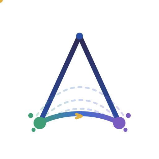






DeltaFlow: optimal-transport flow matching for data-scarce domains
Composable PyTorch primitives for representation learning and posterior sampling, built around the displacement between two distributions.
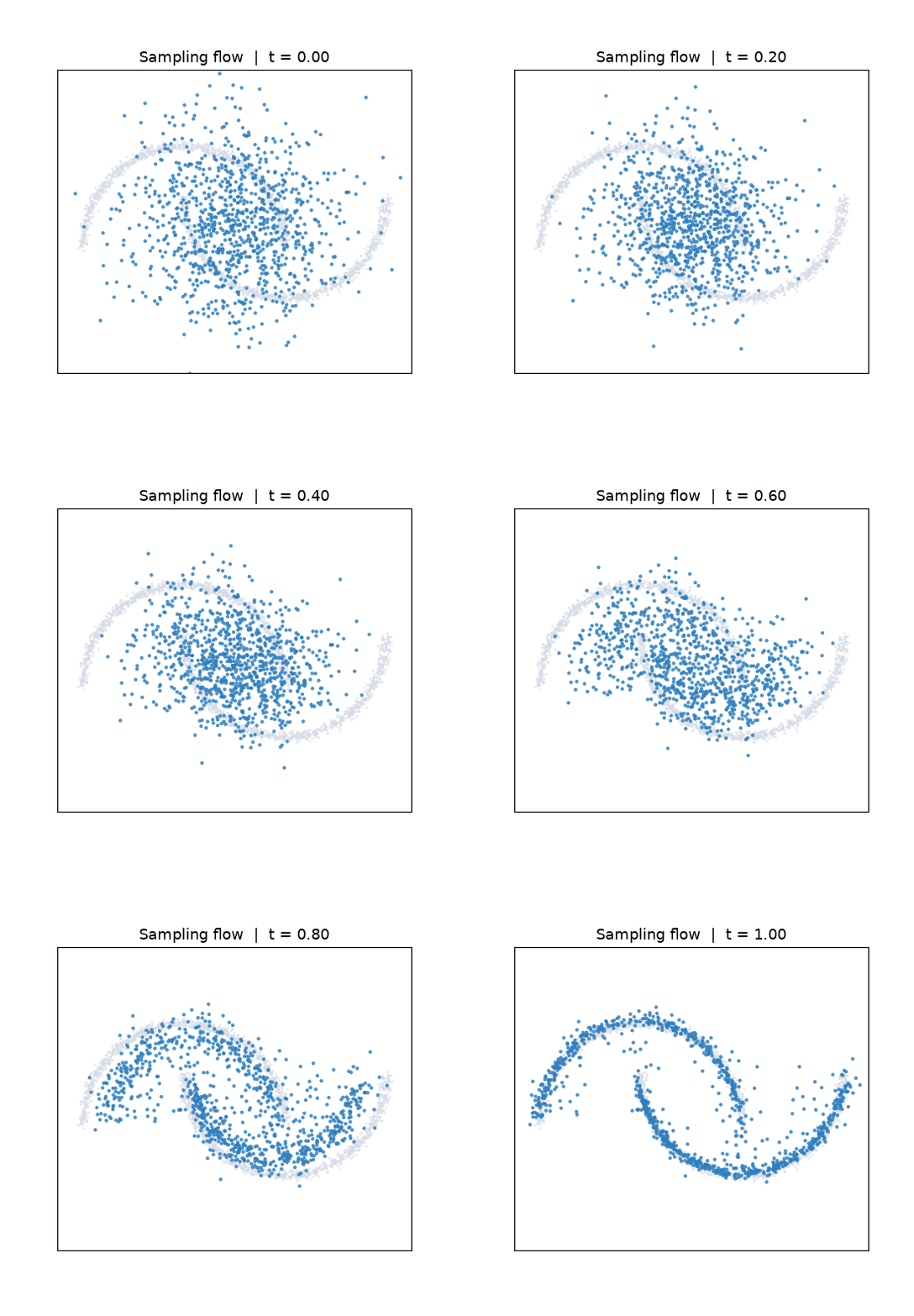
A learned field integrated from noise onto data with FlowSampler.
What is DeltaFlow?
DeltaFlow is a PyTorch library for generative modelling in data-scarce domains such as medical imaging, with a focus on representation learning and studying the underlying data distribution rather than sample synthesis alone. It targets 2D radiography (chest X-ray, cephalometric, and hand radiographs), yet the core primitives stay domain-agnostic.
The whole library follows from one idea, a delta (the change carried from a source distribution to a target one) and the flow that realises it.
- Δ, the change between two distributions. The learning signal is a displacement, $\Delta = x_1 - x_0$, the straight-line velocity that carries a source sample $x_0$ (noise) onto a data sample $x_1$. Regressing a field onto this displacement is exactly the flow-matching objective.
- Flow, integrating the change. A learned field $v_\theta(x, t)$ is integrated as an ODE, $dx/dt = v_\theta(x, t)$, transporting the whole source density onto the data density with a simple Euler or Heun solver.
- Straighter Δ via optimal transport. Which target each source pairs with is a choice. Mini-batch optimal-transport coupling solves the discrete Kantorovich assignment on each batch, so the displacements stay short and the flow stays straight, which is what lets the model sample in fewer steps.
So DeltaFlow implements each component once and lets the method be a configuration.
| Component | The question it answers | Package |
|---|---|---|
| Velocity field | what carries noise onto data? | deltaflow.core, deltaflow.models |
| Interpolant | along which path do noise and data connect? | deltaflow.interpolants |
| Coupling | which noise sample is paired with which datum? | deltaflow.trainer |
| Objective | how is the field fit to data? | deltaflow.losses |
| Solver | which dynamics turn the field into samples? | deltaflow.solvers |
| Inverse | how does one measurement steer sampling? | deltaflow.inverse |
Compose them one way and you have flow matching with an independent coupling. Another way and you have OT-coupled rectified flow. Another and you have posterior sampling for an inverse problem, reusing the very same pretrained field.
Full documentation lives on the DeltaFlow website.
What's inside
Probability paths (deltaflow.interpolants)
The path decides how noise becomes data. Every path returns the interpolated state $x_t$ and its conditional target velocity $u_t$.
| Interpolant | Path |
|---|---|
LinearInterpolant |
straight-line rectified-flow path, $x_t = (1-t)x_0 + t x_1$, $u_t = x_1 - x_0$ |
VariancePreservingInterpolant |
trigonometric diffusion path, $\alpha_t = \sin(\tfrac{\pi}{2}t)$, $\sigma_t = \cos(\tfrac{\pi}{2}t)$ |
OTInterpolant |
the linear path applied after a mini-batch OT re-ordering of $x_0$ |
SchrodingerBridgeInterpolant |
entropic Schrödinger-bridge path, a Brownian bridge $x_t = (1-t)x_0 + t x_1 + \sigma\sqrt{t(1-t)},z$ around the straight line, diffusivity $\sigma$ |
Couplings (deltaflow.trainer)
The coupling decides which noise becomes which datum. Straighter pairings mean straighter paths and fewer sampling steps.
| Coupling | Pairing |
|---|---|
IndependentCoupling |
draw $x_0 \sim \mathcal{N}(0, I)$ independently of $x_1$, the classical setup |
OTCoupling |
permute $x_0$ within the batch to minimise squared transport cost (Hungarian, greedy fallback) |
Objectives (deltaflow.losses)
| Objective | Idea |
|---|---|
FlowMatchingLoss / ConditionalFlowMatchingLoss |
regress $v_\theta(x_t, t)$ onto the path's conditional velocity $u_t$ |
DeltaAlignmentLoss |
align the guidance-difference feature $\Delta h = h_\text{cond} - h_\text{uncond}$ across two views, an anatomy-cancelling representation loss |
Solvers (deltaflow.solvers)
| Solver | Dynamics |
|---|---|
EulerSolver (FlowSampler) |
first-order explicit Euler integration of the flow ODE |
HeunSolver |
second-order Heun integration, more accurate at low step counts |
PosteriorSolver |
wraps any base solver and injects a measurement-likelihood gradient per step |
Inverse problems (deltaflow.inverse)
Measurement operators (MaskOperator, BlurOperator, DownsampleOperator, IdentityOperator), a flow-matching Tweedie decomposition (LinearTweedie, VPTweedie) that recovers a clean-signal estimate from $(x_t, v_t, t)$, and Gaussian likelihoods (GaussianLikelihood) with an optional decoder pullback for the latent-space case.
Install
pip install torchdeltaflow
# or, from source with docs and dev tooling:
pip install -e ".[dev]"
The import name is deltaflow.
Usage
Each block below is one method, in as few lines as it takes. Annotated, full-scale versions live in the examples gallery.
Flow matching
Flow Matching for Generative Modeling, Lipman et al. 2023. Regress a velocity field onto the conditional velocity of a probability path. With DeltaFlow's primitives, that is the loop itself.
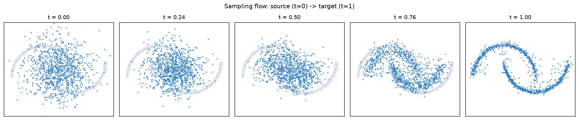
Noise at t=0 reshaped into the two-moons data manifold at t=1. The faint cloud is the target reference.
import torch
from deltaflow.interpolants import LinearInterpolant
from deltaflow.losses import FlowMatchingLoss
from deltaflow.samplers import FlowSampler

loss_fn = FlowMatchingLoss(interpolant=LinearInterpolant())
loss = loss_fn(model, x1)                        # model(x_t, t) -> predicted velocity
loss.backward()

samples = FlowSampler(model).sample(torch.randn(1000, 2), n_steps=50)
Optimal-transport couplings
Improving and generalizing flow-based generative models with minibatch optimal transport, Tong et al. 2024. Pair each noise sample with the right datum and the paths straighten, so generation needs fewer steps. This hard assignment is the zero-entropy limit of the static Schrödinger bridge.
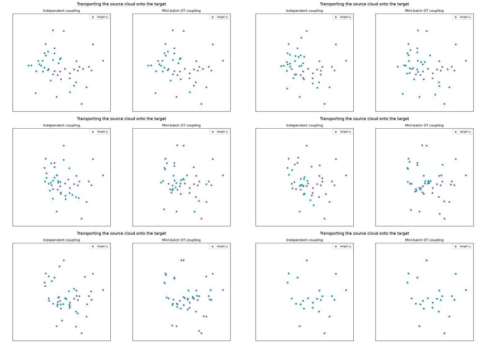
The same source and target clouds under two couplings. The independent pairing sweeps long crossing paths, the OT pairing stays an orderly bundle at lower transport cost.
from deltaflow.losses import ConditionalFlowMatchingLoss
from deltaflow.trainer import OTCoupling

loss_fn = ConditionalFlowMatchingLoss(coupling=OTCoupling())   # same objective, OT pairs
loss = loss_fn(model, x1)
Variance-preserving path
SiT: Exploring Flow and Diffusion-based Generative Models with Scalable Interpolant Transformers, Ma et al. 2024, building on Stochastic Interpolants, Albergo et al. 2023. Swap the interpolant and the same loss and solver run a variance-preserving diffusion path instead of the straight one.
from deltaflow.interpolants import VariancePreservingInterpolant
from deltaflow.losses import FlowMatchingLoss

loss_fn = FlowMatchingLoss(interpolant=VariancePreservingInterpolant())
loss = loss_fn(model, x1)
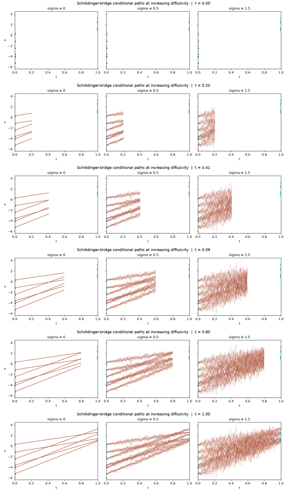
Schrödinger bridge
Diffusion Schrödinger Bridge with Applications to Score-Based Generative Modeling, De Bortoli et al. 2021; Simulation-Free Schrödinger Bridges via Score and Flow Matching (SF2M), Tong et al. 2024. The dynamic Schrödinger bridge between noise and data, conditioned on an endpoint pair, is a Brownian bridge around the straight-line path; regressing onto its conditional velocity trains a stochastic interpolant that recovers the entropic optimal-transport bridge as the coupling of (x0, x1) approaches the true OT plan. Pairing endpoints with OTCoupling (rather than drawing them independently) is what makes this approximation tight in practice.
from deltaflow.interpolants import SchrodingerBridgeInterpolant
from deltaflow.losses import ConditionalFlowMatchingLoss
from deltaflow.trainer import OTCoupling

loss_fn = ConditionalFlowMatchingLoss(
    interpolant=SchrodingerBridgeInterpolant(sigma=1.0),
    coupling=OTCoupling(),
)
loss = loss_fn(model, x1)
Comparing the paths
Every algorithm above is the same training loop; only the interpolant= (and optionally coupling=) argument to ConditionalFlowMatchingLoss changes. Training an identical MLP on a two-moons target with each configuration for the same number of steps makes the differences concrete:
| Path | interpolant= |
coupling= |
|---|---|---|
| Linear (independent) | LinearInterpolant() |
(none, x0 ~ N(0,I)) |
| OT coupling | LinearInterpolant() |
OTCoupling() |
| Variance-preserving | VariancePreservingInterpolant() |
(none) |
| Schrödinger bridge | SchrodingerBridgeInterpolant(sigma=0.5) |
OTCoupling() |
Side by side, animated. All four samplers integrated from the same noise batch, at the same number of steps, so the only difference on screen is the training configuration:
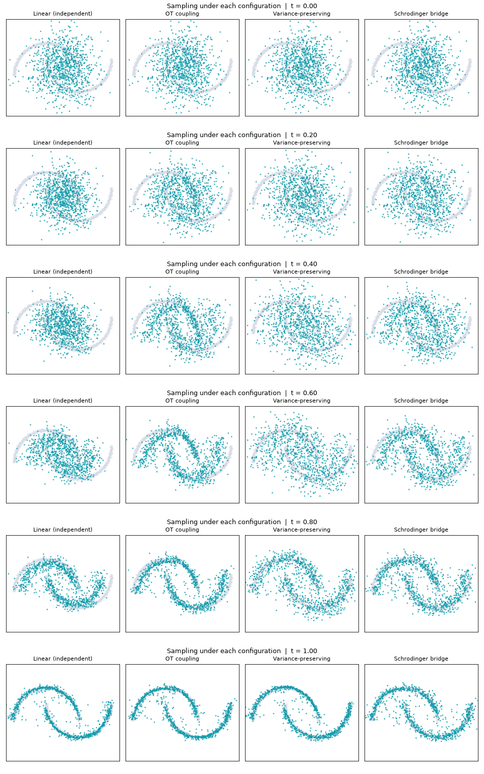
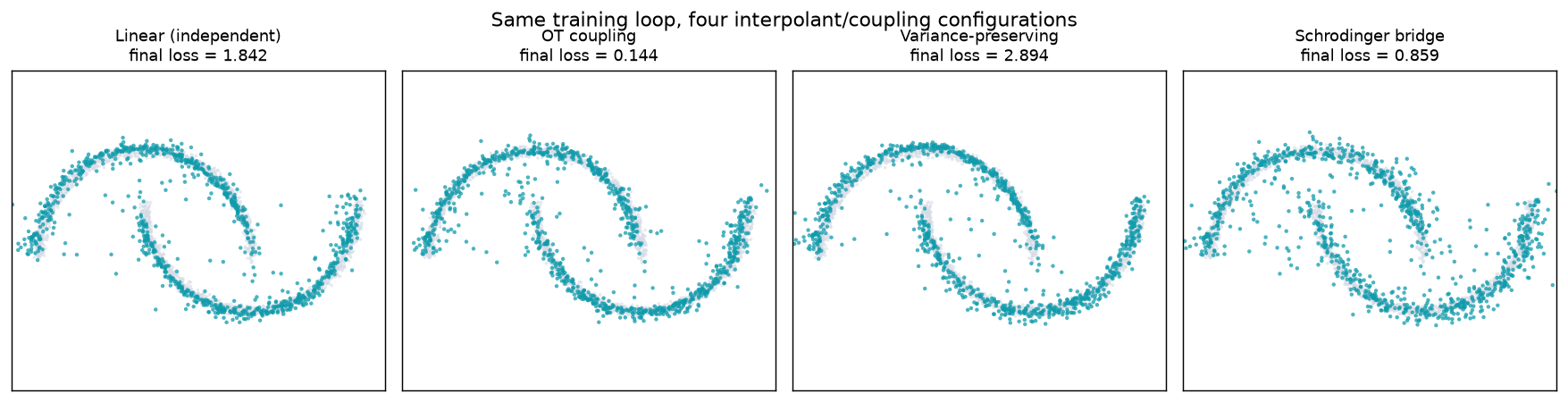
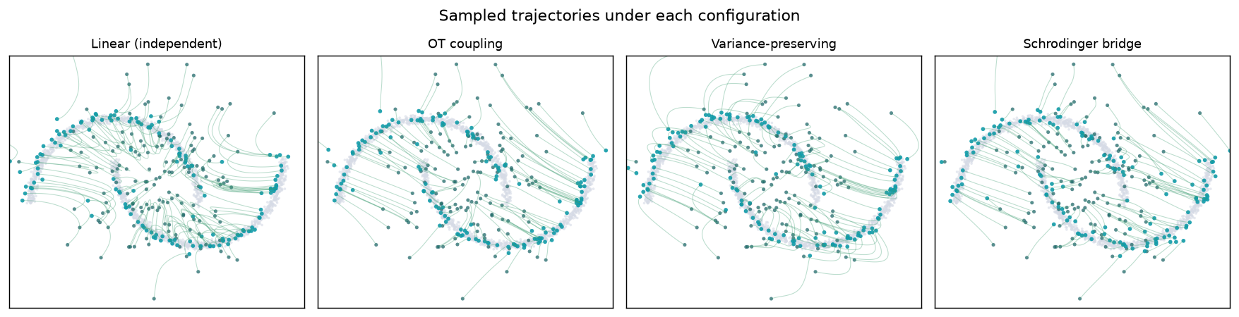
OT coupling produces the straightest source-to-target trajectories of the four (compare the crossing paths on the left to the untangled bundle in the second panel), which is the practical benefit of minimising batch transport cost before regressing. Reproduce this figure with examples/90-showcase/06-algorithm-comparison/.
Delta alignment
The same difference principle powers an optional representation-learning loss. For a conditionally-generated backbone, the guidance-difference feature $\Delta h = h_\text{cond} - h_\text{uncond}$ isolates what the conditioning changed at each hierarchy level, largely cancelling the anatomy both passes share. Aligning $\Delta h$ across two augmented views encourages a guidance representation that is consistent regardless of anatomy. The guidance difference itself follows Classifier-Free Diffusion Guidance, Ho & Salimans 2022.
from deltaflow.losses import DeltaAlignmentLoss
from deltaflow.models import MultiScaleProjector

projector = MultiScaleProjector(feature_dims={"enc_1_4": 256, "bottleneck": 1024})
loss_fn = DeltaAlignmentLoss(projector, lambda_flow=1.0, lambda_align=5.0)

total, loss_dict = loss_fn(
    v_c1, v_u1, target_v1,
    v_c2, v_u2, target_v2,
    feats_u1, feats_c1, feats_u2, feats_c2,
)
Posterior sampling for inverse problems
FlowDPS: Flow-Driven Posterior Sampling for Inverse Problems, Kim et al. 2025, and Flower: A Flow-Matching Solver for Inverse Problems, Pourya et al. 2025. Reconstruct a masked or degraded measurement with a field trained once, no retraining. PosteriorSolver wraps the same Euler solver and injects a measurement-likelihood gradient at every step, so the base integrator is reused rather than re-implemented.
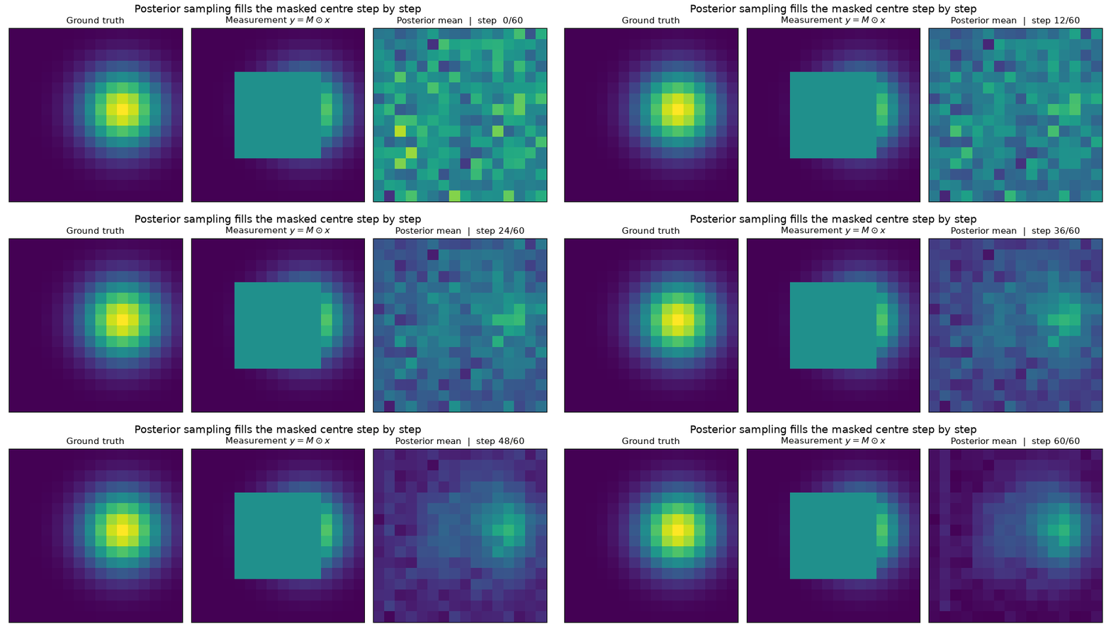
The posterior mean fills a masked centre step by step. The known pixels stay anchored by the likelihood while the flow supplies the rest.
import torch
from deltaflow.inverse import GaussianLikelihood, LinearTweedie, MaskOperator
from deltaflow.solvers import EulerSolver, PosteriorSolver

likelihood = GaussianLikelihood(y=y, operator=MaskOperator(mask), sigma=1.0)
solver = PosteriorSolver(
    base_solver=EulerSolver(model),
    likelihood=likelihood,
    tweedie=LinearTweedie(),
    guidance_scale=0.5,
    grad_normalize=True,
)
x = solver.sample(torch.randn(16, 1, 16, 16), n_steps=60)     # posterior samples
Visualizing the algorithm
Beyond the animations above, examples/90-showcase/02-sampling-flow-viz/ records every intermediate state of a small MLP field trained on a 2D two-moons target.
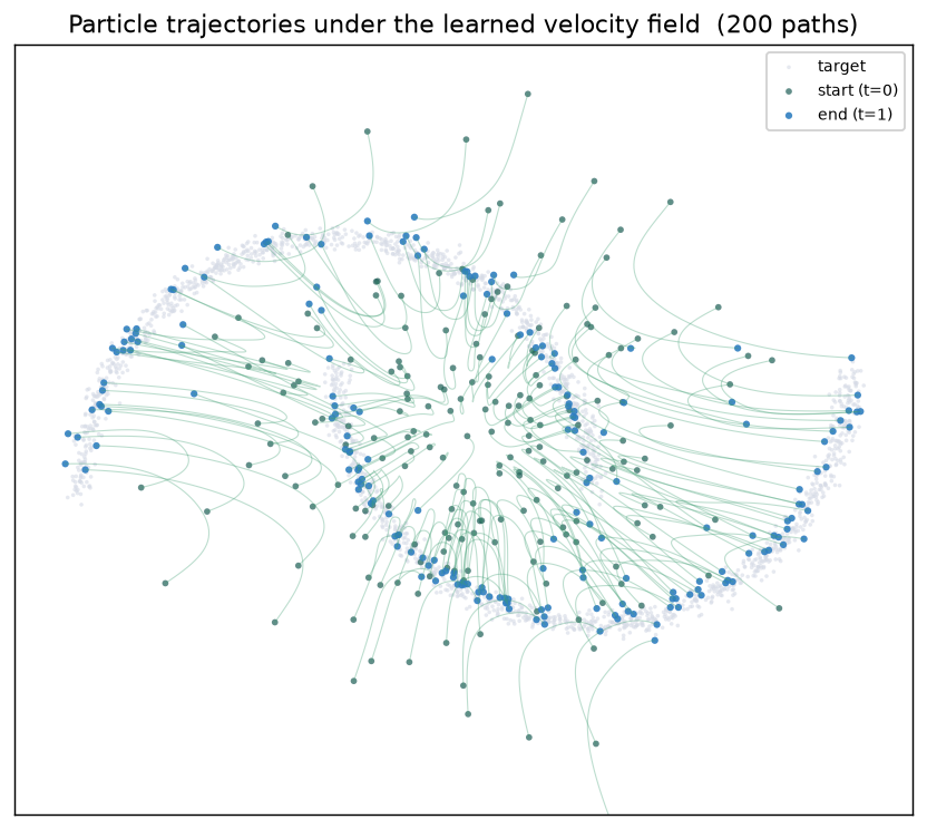
Individual sample paths from noise to data, traced as streamlines.
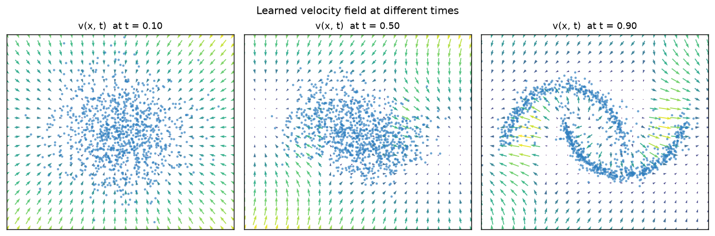
Quiver plots of v(x, t) at three times, pointing broadly inward early on and resolving the two-moons structure by t ≈ 0.9.
Reproduce every figure with:
pip install -e ".[dev]" matplotlib
python examples/90-showcase/02-sampling-flow-viz/main.py     # sampling flow figures and gif
python examples/90-showcase/03-minibatch-ot-viz/main.py      # OT vs independent coupling
python examples/90-showcase/04-inverse-posterior-viz/main.py # posterior reconstruction
python examples/90-showcase/07-landmark-detection/main.py    # landmark detection as conditional flow
python examples/90-showcase/08-guidance-alignment-pretraining/main.py # guidance-aligned pretraining
Landmark detection and representation learning
Two paired showcases cover the anatomical-landmark story. 07-landmark-detection/ frames detection as a conditional flow p(landmarks | image), so sampling at inference time is detection (synthetic by default, with real ISBI2015 cephalometric support). 08-guidance-alignment-pretraining/ is the representation-learning counterpart, the CDPM-Align pretraining phase, where a class-conditioned image flow plus the DeltaAlignmentLoss over Δh = h_cond − h_uncond yields an anatomy-discriminative backbone.
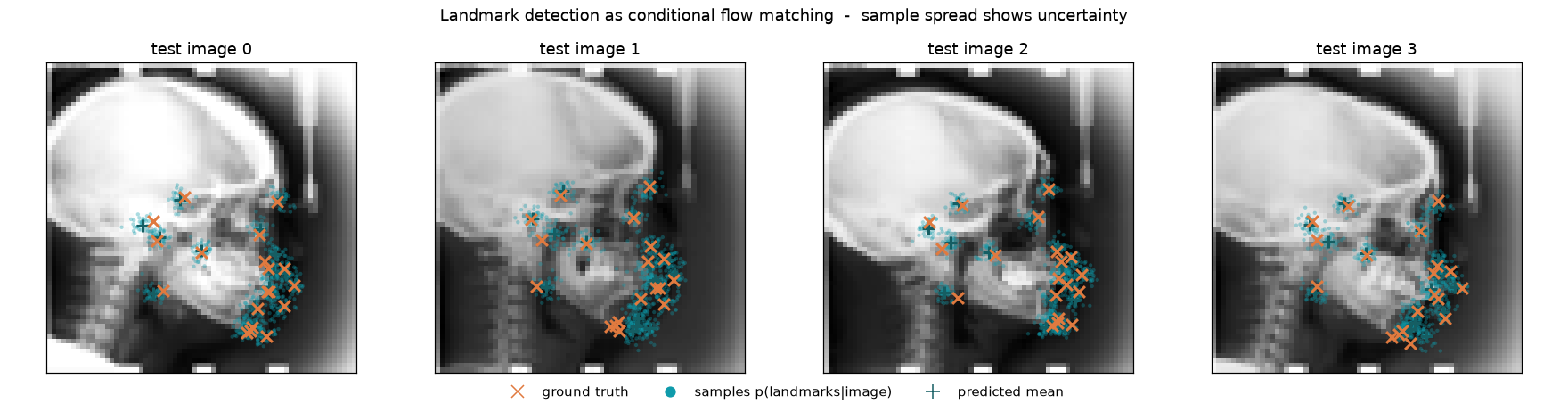
Detection as posterior sampling. Orange crosses are ground truth, teal dots are samples from p(landmarks | image), and teal pluses are the predicted means. Sample spread is a built-in uncertainty estimate.
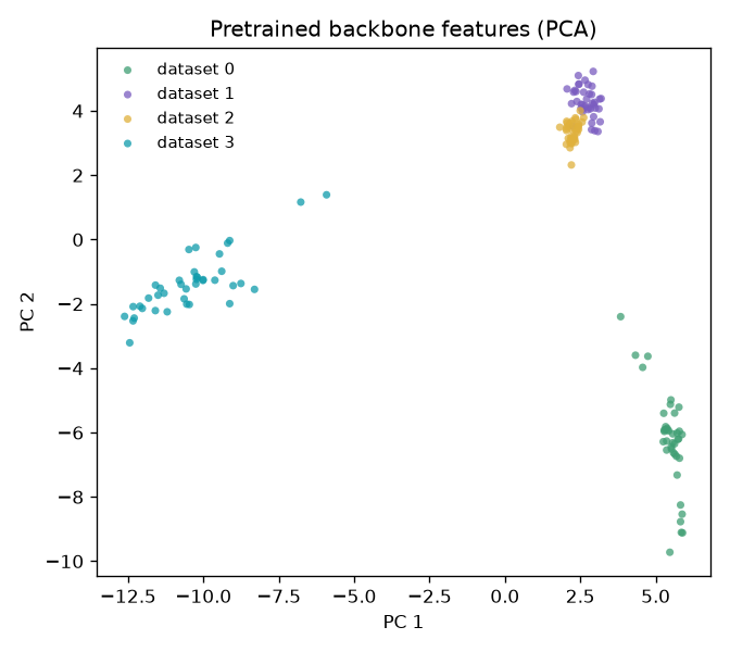
PCA of the frozen backbone features on held-out images. The four synthetic datasets separate cleanly, so a linear probe recovers dataset identity trivially, evidence that guided generative pretraining learned an anatomy-discriminative representation.
Examples
The examples/ tree is a tiered, runnable curriculum.
| Tier | You learn to |
|---|---|
00-foundations/ |
work with interpolants and the linear probability path |
10-sampling/ |
integrate a learned field with the Euler and Heun solvers |
20-training/ |
fit a field with flow matching, OT coupling, and delta alignment |
90-showcase/ |
study end-to-end demos and the visualizations above, including the Schrödinger-bridge path and trained sampler, the four-algorithm comparison, landmark detection as conditional flow, and guidance-aligned representation pretraining |
Development
pip install -e ".[dev]"
pytest
Contributing
Contributions are welcome. Please read CONTRIBUTING.md before getting started.
Citation
If DeltaFlow is useful in your research, please cite it (see CITATION.cff):
@misc{deltaflow_library_2025,
  author = {Limbunlom, Phrugsa},
  title  = {{DeltaFlow}: Optimal-Transport Flow Matching for Data-Scarce Domains in {PyTorch}},
  year   = {2025},
  url    = {https://github.com/phrugsa-limbunlom/deltaflow},
}
Citations
DeltaFlow builds on the following work.
@inproceedings{lipman2023flow,
  title  = {Flow Matching for Generative Modeling},
  author = {Lipman, Yaron and Chen, Ricky T. Q. and Ben-Hamu, Heli and Nickel, Maximilian and Le, Matt},
  year   = {2023},
  eprint = {2210.02747},
  url    = {https://arxiv.org/abs/2210.02747},
}
@inproceedings{liu2023flow,
  title  = {Flow Straight and Fast: Learning to Generate and Transfer Data with Rectified Flow},
  author = {Liu, Xingchao and Gong, Chengyue and Liu, Qiang},
  year   = {2023},
  eprint = {2209.03003},
  url    = {https://arxiv.org/abs/2209.03003},
}
@article{albergo2023stochastic,
  title  = {Stochastic Interpolants: A Unifying Framework for Flows and Diffusions},
  author = {Albergo, Michael S. and Boffi, Nicholas M. and Vanden-Eijnden, Eric},
  year   = {2023},
  eprint = {2303.08797},
  url    = {https://arxiv.org/abs/2303.08797},
}
@article{ma2024sit,
  title  = {SiT: Exploring Flow and Diffusion-based Generative Models with Scalable Interpolant Transformers},
  author = {Ma, Nanye and Goldstein, Mark and Albergo, Michael S. and Boffi, Nicholas M. and Vanden-Eijnden, Eric and Xie, Saining},
  year   = {2024},
  eprint = {2401.08740},
  url    = {https://arxiv.org/abs/2401.08740},
}
@article{tong2024improving,
  title   = {Improving and generalizing flow-based generative models with minibatch optimal transport},
  author  = {Tong, Alexander and Fatras, Kilian and Malkin, Nikolay and Huguet, Guillaume and Zhang, Yanlei and Rector-Brooks, Jarrid and Wolf, Guy and Bengio, Yoshua},
  journal = {Transactions on Machine Learning Research},
  year    = {2024},
  eprint  = {2302.00482},
  url     = {https://arxiv.org/abs/2302.00482},
}
@inproceedings{ho2022classifier,
  title  = {Classifier-Free Diffusion Guidance},
  author = {Ho, Jonathan and Salimans, Tim},
  year   = {2022},
  eprint = {2207.12598},
  url    = {https://arxiv.org/abs/2207.12598},
}
@inproceedings{kim2025flowdps,
  title  = {FlowDPS: Flow-Driven Posterior Sampling for Inverse Problems},
  author = {Kim, Jeongsol and Kim, Bryan Sangwoo and Ye, Jong Chul},
  year   = {2025},
  eprint = {2503.08136},
  url    = {https://arxiv.org/abs/2503.08136},
}
@article{pourya2025flower,
  title  = {Flower: A Flow-Matching Solver for Inverse Problems},
  author = {Pourya, Mehrsa and El Rawas, Bassam and Unser, Michael},
  year   = {2025},
  eprint = {2509.26287},
  url    = {https://arxiv.org/abs/2509.26287},
}
@article{debortoli2021diffusion,
  title  = {Diffusion Schr{\"o}dinger Bridge with Applications to Score-Based Generative Modeling},
  author = {De Bortoli, Valentin and Thornton, James and Heng, Jeremy and Doucet, Arnaud},
  year   = {2021},
  eprint = {2106.01357},
  url    = {https://arxiv.org/abs/2106.01357},
}
@article{tong2024simulationfree,
  title   = {Simulation-Free Schr{\"o}dinger Bridges via Score and Flow Matching},
  author  = {Tong, Alexander and Malkin, Nikolay and Fatras, Kilian and Atanackovic, Lazar and Zhang, Yanlei and Huguet, Guillaume and Wolf, Guy and Bengio, Yoshua},
  year    = {2024},
  eprint  = {2307.03672},
  url     = {https://arxiv.org/abs/2307.03672},
}
License
MIT. See LICENSE.
1 maintainer

Download files
Download the file for your platform. If you're not sure which to choose, learn more about installing packages.
Source Distribution
Built Distribution
Filter files by name, interpreter, ABI, and platform.
If you're not sure about the file name format, learn more about wheel file names.
Copy a direct link to the current filters
File details
Details for the file torchdeltaflow-0.2.2.tar.gz.
File metadata
- Download URL: torchdeltaflow-0.2.2.tar.gz
- Upload date:
- Size: 12.8 MB
- Tags: Source
- Uploaded using Trusted Publishing? No
- Uploaded via:
twine/7.0.0 CPython/3.13.14
File hashes
| Algorithm | Hash digest | |
|---|---|---|
| SHA256 |
3af84023dbc0180ea72aff302feea5e45ca4849b86e91a04bd39e92457def2ef
|
|
| MD5 |
8e35ad1a87220a0005ebd9a30a334002
|
|
| BLAKE2b-256 |
d9ebd2d5da6cf06f18e55d4d961f0e5f1dc0a69d05501aaabc65fea105388547
|
File details
Details for the file torchdeltaflow-0.2.2-py3-none-any.whl.
File metadata
- Download URL: torchdeltaflow-0.2.2-py3-none-any.whl
- Upload date:
- Size: 54.5 kB
- Tags: Python 3
- Uploaded using Trusted Publishing? No
- Uploaded via:
twine/7.0.0 CPython/3.13.14
File hashes
| Algorithm | Hash digest | |
|---|---|---|
| SHA256 |
04b5439d75743d42bd379d04fafb2ff4ae54452da43beff47868ae9634e5d0d9
|
|
| MD5 |
370d4f36493eea712ad14685a7162f91
|
|
| BLAKE2b-256 |
087ea2959e88a89a035e48995a9bdb8f0f2464a7fca99ddb6f7fe2ead5b7e598
|














