





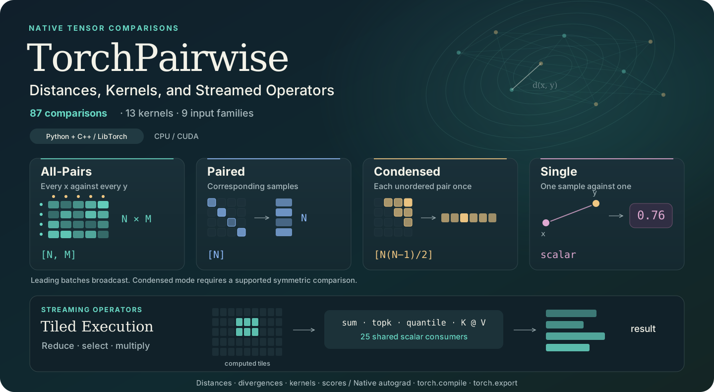
Compare tensors with one API, whether a sample is a vector, a point cloud, an image, a waveform or a distribution. Return the comparisons themselves, or stream the result your algorithm needs through reductions, neighbor selection and matrix products. Python and standalone C++/LibTorch share native forward and first-backward implementations on CPU and CUDA.


Comparison modes · Streaming operators · C++ / LibTorch · Build from source · Full comparison catalog
The documentation website organizes metrics by equation, input/output shape and comparison mode, with Python/C++ examples. Local preview and website builds use mdBook.
| Choose your result | API | What it produces |
|---|---|---|
| Every sample pair | compare(X, Y, mode="all_pairs", ...) |
[..., N, M] |
| Corresponding samples | compare(X, Y, mode="paired", ...) |
[..., N] |
| Each unordered self pair once | compare(X, mode="condensed", ...) |
[..., N*(N-1)//2], for supported symmetric comparisons |
| One sample pair per batch | compare(x, y, mode="single", ...) |
[...]; a scalar without batches |
| A reduced, selected or multiplied result | tp.lazy(...).sum(...), .topk(...), .matmul(V) |
The requested result, without retaining the full generated comparison matrix |
The catalog contains 87 comparison entries, including 13 kernels, across 9 input families. Scalar streaming operators share 25 consumers, with products, selection, basic reductions and statistics. Catalog entries include mathematical synonyms; counts describe the API rather than distinct formulas. Feature residuals and image maps also have streamed event-axis reductions.
Version 1.0. This README describes the 1.0 API. If PyPI still offers 0.3, build from source to use the new features. Native wheels require their matching PyTorch minor. See source builds, migration and release notes.
Quick Start: Four Modes, One Selector
import torch
import torchpairwise as tp

X = torch.randn(20, 6)
Y = torch.randn(30, 6)
metric = "sqeuclidean"

matrix = tp.compare(X, Y, metric=metric)                       # [20, 30]
aligned = tp.compare(X, Y[:20], metric=metric, mode="paired")  # [20]
unordered = tp.compare(X, metric=metric, mode="condensed")     # [190]
value = tp.compare(X[0], Y[0], metric=metric, mode="single")   # scalar
single is a mode of compare. single_comparison(x, y, metric=...) is
an optional shorthand for that same call. Inputs omit the collection's N/M axis:
a vector is [D], a cloud [P,D], an image [C,H,W], and a Gaussian is
(mean[D], covariance[D,D]). Leading batches broadcast in every mode; for
example, single mode on [B,D] vectors returns [B] rather than [B,B].
Use list_comparisons() to discover names, roles, layouts and supported modes.
Most numeric comparisons support first input gradients; Boolean/equality inputs are nondifferentiable. Feature weights can have gradients where their formulas permit. Autocast and compile/export support follow each operation's contract; see API contracts and PyTorch integration.
Keep the Result, Stream the Comparisons
Use tp.lazy to bind comparisons and their consumers. Custom metric and
encoder factories can also supply comparisons to tp.lazy.
Bind a logical comparison matrix, then ask for what you need. A consumer computes sample tiles and combines their results; it does not retain the full generated N-by-M matrix. The same source can feed reductions, selections or products:
V = torch.randn(30, 4)
A = tp.lazy(X, Y, metric="sqeuclidean", chunk_size=16)

nearest = A.topk(3, largest=False)        # values / indices: [20, 3]
row_spread = A.std(dim=-1, correction=0)  # [20]
smoothed = (-0.5 * A).softmax_matmul(V)   # [20, 4]

K = tp.lazy(X, Y, metric="rbf", gamma=0.2)
features = K.matmul(V)  # [20, 4], streamed K @ V
Each consumer recomputes the source tiles; binding an operator does not cache
a matrix. Inputs, prepared features, outputs and gradient buffers still occupy
memory, and some consumers need additional workspace. Chunk widths control
sample or feature tiles, not a total memory budget. They accept any positive
Python integer up to 2**63 - 1, including non-powers of two. See the
streaming guide, selection/statistics
and reproducible benchmarks.
For complete consumers, see the k-NN regression, kernel smoothing and attention
examples, each checked against its dense formula.
The same comparison selector is available in standalone C++:
#include <torchpairwise.h>

namespace tp = torchpairwise::ops;
auto matrix = tp::compare(X, Y, "sqeuclidean", "all_pairs");
auto value = tp::compare(x, y, "sqeuclidean", "single");
See the native API and CMake package for headers, linking, structured inputs, options and native operator consumers.
Implemented Comparisons
Function names below are public exports of torchpairwise. Distances,
divergences, kernels, and quality scores retain their own definitions: a
symmetric comparison is not necessarily a triangle-inequality metric, and an
image similarity score is not automatically a positive-semidefinite kernel.
Aliases are identified explicitly rather than counted as additional formulas.
Vector Geometry and Numeric Data
Inputs normally have shape [..., N, D] and [..., M, D].
| Comparison | Public function | Parameters / convention |
|---|---|---|
| Euclidean | euclidean_distances |
Optional feature weights w |
| Squared Euclidean | sqeuclidean_distances |
Optional w |
| Manhattan | manhattan_distances |
Optional w |
| Minkowski | minkowski_distances |
Power p, optional w |
| Weighted Minkowski | wminkowski_distances |
Legacy weighted-Lp entry point; p, w |
| Chebyshev | chebyshev_distances |
Optional w selects positive-weight coordinates |
| Standardized Euclidean | seuclidean_distances |
Variances V |
| Mahalanobis | mahalanobis_distances |
Inverse covariance VI |
| Cosine distance | cosine_distances |
Optional w |
| Correlation distance | correlation_distances |
Optional w |
| Angular | angular_distances |
Radians; nonzero vectors |
| Canberra | canberra_distances |
Optional w |
| Bray-Curtis | braycurtis_distances |
Optional w |
| Lorentzian | lorentzian_distances |
Sum of log1p absolute differences |
| Haversine | haversine_distances |
Latitude/longitude in radians, D=2 |
| Signal-to-noise ratio | snr_distances |
Directed comparison |
| NaN-aware Euclidean | nan_euclidean_distances |
Missing-feature rescaling; optional squared |
| Alias | Equivalent entry point |
|---|---|
l1_distances, cityblock_distances |
manhattan_distances |
l2_distances |
euclidean_distances |
lp_distances |
minkowski_distances |
linf_distances |
chebyshev_distances |
See feature weighting, angular and related distances, and missing-data comparisons.
Boolean and Equality Comparisons
Hamming compares equality of numeric or Boolean coordinates. The other entries
use Boolean vectors. Each accepts optional feature weights w; input
comparisons themselves have no derivatives. Undefined empty-support cases and
weight-gradient conventions are described in the
contracts and weighting guide.
| Comparison | Public function |
|---|---|
| Hamming | hamming_distances |
| Jaccard | jaccard_distances |
| Dice | dice_distances |
| Yule | yule_distances |
| Rogers-Tanimoto | rogerstanimoto_distances |
| Russell-Rao | russellrao_distances |
| Sokal-Michener | sokalmichener_distances |
| Sokal-Sneath | sokalsneath_distances |
| Kulczynski1 | kulczynski1_distances |
| Legacy Kulsinski | kulsinski_distances |
Histograms, Probabilities, and Compositions
These use one dense vector per sample. The normalization/domain column matters: raw masses, probability distributions, and positive compositions have different meanings. Domain and zero/infinite-support gradient conventions are in the histogram, probability, and composition guides.
| Comparison | Public function | Normalization / domain |
|---|---|---|
| Hellinger | hellinger_distances |
Independently normalized nonnegative positive-mass rows |
| Bhattacharyya distance | bhattacharyya_distances |
Normalized; negative log coefficient |
| Total variation | total_variation_distances |
Normalized; half L1 |
| Fisher-Rao | fisher_rao_distances |
Normalized; twice the square-root probability angle |
| Jensen-Shannon distance | jensenshannon_distances |
Normalized; rooted divergence; optional log base |
| KL divergence | kl_divergences |
Normalized; directed; optional base |
| Symmetric KL / Jeffreys | symmetric_kl_divergences |
Normalized; sum of both KL directions |
| Rényi divergence | renyi_divergences |
Normalized; positive finite alpha, KL at one |
| Pearson chi-square | pearson_chi2_divergences |
Normalized; second operand in denominator |
| Neyman chi-square | neyman_chi2_divergences |
Normalized; first operand in denominator |
| Triangular discrimination | triangular_discrimination_distances |
Normalized; no half factor |
| Itakura-Saito | itakura_saito_divergences |
Raw strictly positive spectra |
| Aitchison | aitchison_distances |
Strictly positive compositions; centered log-ratios |
| Clark | clark_distances |
Raw nonnegative vectors; coordinate-wise relative differences |
| Soergel / Ružička | soergel_distances, ruzicka_distances |
Same continuous min/max Jaccard formula for raw nonnegative vectors |
| Continuous Jaccard alias | continuous_jaccard_distances |
Alias of ruzicka_distances; distinct from Boolean Jaccard |
| Shared-grid 1D Wasserstein | wasserstein_1d_distances |
Normalized histogram masses; optional ordered bin_positions |
Point Sets and Empirical Distributions
A sample is a collection of points: standard inputs are [..., N, P, C] and
[..., M, Q, C]. Spatial feature axes, channel-first layouts, prefix lengths,
and sample chunking follow the point-set guide.
| Comparison | Public function | Convention |
|---|---|---|
| Directed Hausdorff | directed_hausdorff_distances |
Returns distances and point witnesses; asymmetric |
| Symmetric Hausdorff | hausdorff_distances |
Maximum of the two directed Euclidean distances |
| Chamfer | chamfer_distances |
Sum of directional mean nearest-point distances; optional squared |
| Exact multidimensional Wasserstein | wasserstein_distances |
Uniform empirical W1/W2; p=1 or 2; CPU-coordinated solver, including CUDA inputs |
| Sliced Wasserstein | sliced_wasserstein_distances |
Uniform projected W1/W2; explicit shared projections |
| Sinkhorn divergence | sinkhorn_divergences |
Debiased regularized transport estimate; fixed iteration budget |
| Energy distance | energy_distances |
Uniform empirical V statistic; rooted by default |
| Kernel MMD | mmd_distances |
Biased V statistic; 11 named registry kernels plus historical Euclidean Laplacian; polynomial options supported; rooted by default |
| MMD estimates / KID statistic | mmd_statistics |
Signed biased/unbiased estimates; selectable kernels including cubic polynomial on supplied features; no learned model |
Transport compares uniform point masses; it is separate from histogram-bin
wasserstein_1d_distances. Exact transport is intended for small clouds. Sliced
Wasserstein and finite-iteration Sinkhorn retain their distinct approximation
and gradient contracts. See transport,
distribution comparisons, and the
example.
Gaussian Distributions and Covariance Geometry
These standalone structured APIs use explicit means/covariances or covariance
matrices. They are separate from the vector cdist/pdist registry. Each row
has all three output modes; squared=True selects the unrooted quantity.
| Comparison | All-pairs function | Paired function | Condensed function |
|---|---|---|---|
| Gaussian Wasserstein / Bures W2 | gaussian_wasserstein_distances |
paired_gaussian_wasserstein_distances |
condensed_gaussian_wasserstein_distances |
| Log-Euclidean covariance distance | log_euclidean_distances |
paired_log_euclidean_distances |
condensed_log_euclidean_distances |
| Affine-invariant Riemannian covariance distance | affine_invariant_distances |
paired_affine_invariant_distances |
condensed_affine_invariant_distances |
| Rooted Stein / Jensen-Bregman LogDet | stein_distances |
paired_stein_distances |
condensed_stein_distances |
Gaussian W2 accepts means [..., N, D] and positive-semidefinite covariances
[..., N, D, D]. The other three require strictly positive-definite covariances.
See Gaussian comparisons and
covariance geometry for tolerances, singular
boundaries, memory, and first-gradient support.
Gaussian Mixtures and Splat Geometry
Each sample is a weighted mixture: means [...,N,K,D], covariances
[...,N,K,D,D] and weights [...,N,K]. Explicit masses are normalized per
sample; prefix lengths ignore padding. Density comparisons require SPD
covariances; Gaussian-component transport accepts PSD covariances.
| Comparison | All-pairs function | Paired function | Condensed function |
|---|---|---|---|
| Density overlap | gaussian_mixture_overlap_kernel |
paired_gaussian_mixture_overlap_kernel |
condensed_gaussian_mixture_overlap_kernel |
| Density L2 | gaussian_mixture_l2_distances |
paired_gaussian_mixture_l2_distances |
condensed_gaussian_mixture_l2_distances |
| Cauchy-Schwarz divergence | gaussian_mixture_cauchy_schwarz_divergences |
paired_gaussian_mixture_cauchy_schwarz_divergences |
condensed_gaussian_mixture_cauchy_schwarz_divergences |
| Component Mixture W2 | gaussian_mixture_wasserstein_distances |
paired_gaussian_mixture_wasserstein_distances |
condensed_gaussian_mixture_wasserstein_distances |
| Full entropic transport cost | gaussian_mixture_entropic_transport_costs |
paired_gaussian_mixture_entropic_transport_costs |
condensed_gaussian_mixture_entropic_transport_costs |
| Debiased mixture Sinkhorn | gaussian_mixture_sinkhorn_divergences |
paired_gaussian_mixture_sinkhorn_divergences |
condensed_gaussian_mixture_sinkhorn_divergences |
Component W2 uses an exact small weighted discrete solver controlled by the CPU, including for CUDA inputs; it generally differs from exact W2 between mixture densities. Regularized costs/divergences use fixed iteration budgets. Splat opacity is not automatically mixture mass, and geometry does not measure view-dependent appearance. See Gaussian mixtures and the example.
Ordered Sequences and Integer Tokens
Continuous sequences use [...,N,T,D], with optional valid prefix lengths and
a warping window. Integer tokens use [...,N,T], with user-owned tokenization;
their int64 edit counts have no input derivatives. Batch axes broadcast.
| Comparison | All-pairs function | Paired function | Condensed function |
|---|---|---|---|
| Dynamic time warping | dtw_distances |
paired_dtw_distances |
condensed_dtw_distances |
| Debiased Soft-DTW | soft_dtw_divergences |
paired_soft_dtw_divergences |
condensed_soft_dtw_divergences |
| Levenshtein | levenshtein_distances |
paired_levenshtein_distances |
condensed_levenshtein_distances |
| Insertion/deletion / LCS | indel_distances |
paired_indel_distances |
condensed_indel_distances |
DTW uses squared Euclidean frame costs and optionally returns their rooted
alignment sum. Soft-DTW divergence takes explicit gamma and remains unrooted
and unclamped. Indel equals the two sequence lengths minus twice their longest
common subsequence length. See continuous sequences
and tokens.
Kernels and Vector Similarities
These use pairwise_kernels, paired_kernels, and condensed_kernels, with
kernel-specific parameters. See the kernel,
histogram, and distribution
guides for formulas and domains.
| Kernel / similarity | Public function | Main options / convention |
|---|---|---|
| Linear | linear_kernel |
Dot product |
| Polynomial | polynomial_kernel |
degree, gamma, coef0 |
| Sigmoid | sigmoid_kernel |
gamma, coef0 |
| Gaussian RBF | rbf_kernel |
gamma; squared Euclidean ground distance |
| Laplacian | laplacian_kernel |
gamma; Manhattan ground distance |
| Rational quadratic | rational_quadratic_kernel |
length_scale, alpha |
| Matérn | matern_kernel |
length_scale; nu=0.5, 1.5, or 2.5 |
| Cosine similarity | cosine_similarity |
Normalized dot product |
| Additive chi-square | additive_chi2_kernel |
Nonnegative vectors |
| Exponentiated chi-square | chi2_kernel |
Nonnegative vectors; gamma |
| Histogram intersection | histogram_intersection_kernel |
Sum of coordinate minima of raw nonnegative masses |
| Bhattacharyya coefficient | bhattacharyya_kernel |
Independently normalized histogram rows |
Aligned Image Quality Scores
Inputs are whole aligned images [..., N, C, H, W], with explicit data_range.
Higher scores mean greater similarity. These standalone score APIs follow the
image comparison guide, including SSIM window,
MS-SSIM pooling/weighting, identity, precision, and gradient conventions.
| Score | All-pairs function | Paired function | Condensed function |
|---|---|---|---|
| PSNR | psnr_scores |
paired_psnr_scores |
condensed_psnr_scores |
| SSIM | ssim_scores |
paired_ssim_scores |
condensed_ssim_scores |
| MS-SSIM | multiscale_ssim_scores |
paired_multiscale_ssim_scores |
condensed_multiscale_ssim_scores |
Learned encoders and weights stay in user code. Gaussian W2 squared supplies the
Gaussian feature-moment comparison used by FID; this is not an image-to-FID
pipeline. LPIPS/DISTS models and an image-to-KID pipeline are not provided;
mmd_statistics supplies the KID-style polynomial estimator on caller-supplied
features. See learned representations.
Aligned Audio Quality and Spectra
Inputs use [...,N,C,T]; channels/time must match. Scores use the second
operand as reference. Spectral options explicitly control FFT/window/hop,
padding and floors. STFT features are reused across partners within a call.
| Comparison | All-pairs function | Paired function | Condensed function |
|---|---|---|---|
| SI-SDR score | si_sdr_scores |
paired_si_sdr_scores |
Directed; unavailable |
| Signal SNR score | signal_snr_scores |
paired_signal_snr_scores |
Directed; unavailable |
| Natural-log spectral L1 | log_spectral_distances |
paired_log_spectral_distances |
condensed_log_spectral_distances |
| Spectral convergence | spectral_convergence_distances |
paired_spectral_convergence_distances |
Directed; unavailable |
| Multi-resolution STFT discrepancy | multiresolution_stft_distances |
paired_multiresolution_stft_distances |
Directed; unavailable |
Floors give finite perfect/silent signal scores and affect scale invariance
near silence. Signal SNR is distinct from vector snr_distances. Spectral
convergence is reference-normalized; multi-resolution discrepancy averages
convergence plus log-magnitude L1. See audio comparisons.
Selectors, Named Functions, and Custom Comparisons
compare(..., metric=..., mode=...) is the common entry for all four modes.
Named functions such as euclidean_distances keep their all-pairs meaning;
paired_ and condensed_ variants are available for selected named functions.
Existing role-specific selectors are useful when the application explicitly
expects distances or kernels:
| Mode | Distances / divergences / costs | Kernels / similarities |
|---|---|---|
| All pairs | pairwise_distances(X,Y,metric=...) / cdist |
pairwise_kernels(X,Y,kernel=...) |
| Paired | paired_distances(X,Y,metric=...) |
paired_kernels(X,Y,kernel=...) |
| Condensed | condensed_distances(X,metric=...) / pdist |
condensed_kernels(X,kernel=...) |
Single comparisons use compare(...,mode="single") for every role; the
single_comparison shorthand uses the same native path. We do not add a separate
single-function variant of every named metric.
Generic registry keys normally match the function stem: angular_distances
uses metric="angular", kl_divergences uses metric="kl", and
matern_kernel uses kernel="matern". Kernel and distance registries are
separate. compare(..., metric=..., mode=...) selects across all families,
including Gaussian, covariance, mixture, image, audio, sequence and token inputs.
Distance selectors now cover all 68 catalog distances/divergences/costs; kernel
selectors cover all 13 kernels. Python and native cdist/pdist share coverage
and parameter validation. compare additionally covers scores/statistics.
See all-family dispatch and single samples.
Condensed distance output excludes asymmetric API entries: snr,
directed_hausdorff, kl, renyi, pearson_chi2, neyman_chi2, and
itakura_saito. All-pairs and paired outputs remain available for them.
Named directed Hausdorff returns witnesses; every generic selector returns one
value Tensor. compare(...,mode="single") and single_comparison omit the N/M
axis and broadcast leading batches. A vector is [D], a point cloud [P,D],
an image [C,H,W], or a Gaussian (mean[D],covariance[D,D]). Single mode reuses
native paired execution; named metrics keep their existing all-pairs meaning.
The experimental make_pairwise factory adapts a pure two-sample scalar
PyTorch function to all four modes, including image-shaped samples, with
optional torch.compile, explicit Tensor parameters and custom VJPs. Its
tp.lazy(X, Y, metric) binds the same formula to scalar streaming and algebra.
C++ make_pairwise also accepts lambdas, function pointers and std::function,
with .expression(X,Y) for streaming. Named native paired-tile operators remain
available for explicit deployment registrations.
Condensed output requires explicit symmetry;
see custom comparisons and the
example. It does not automatically cache learned
features or load models.
make_feature_pairwise(encoder, comparison, ...) composes the user's loaded
encoder with a collection comparison, encoding each original collection once
per call and reusing its features. Use .encode or .prepare for explicit
reuse across heads/consumers, or tp.lazy(X, Y, comparison) to encode once and stream the head.
It preserves the caller's model/gradient settings. See feature reuse
and the example.
For a consistent choice of names, modes and streaming entry points, see the API naming guide.
Streaming Operators
Use tp.lazy in Python and torchpairwise::streaming in C++.
See the migration guide.
Bind a source, optionally combine its entries, then run a consumer. Bindings store tensor references and options; they do not compute or cache the matrix. A later consumer sees input mutations and recomputes the required tiles.
| Source | Logical shape | Coverage / purpose |
|---|---|---|
tp.lazy(X,Y,metric=...) |
[...,N,M] |
All 87 named scalar comparisons, including structured, modality and ordered families |
tp.lazy(X,Y,metric=...) |
[...,N,M] |
13 kernels, with vector geometry methods |
tp.as_lazy(scores) |
[...,N,M] |
Common consumers for a caller-owned dense matrix |
tp.lazy(X,Y,custom) |
[...,N,M] |
User-defined scalar comparisons, with shared algebra/consumers and tile replay |
Scalar expressions such as 0.7*K1 + 0.3*K2 |
[...,N,M] |
Lazy scalar entry algebra across sources |
tp.residual_operator(X,Y,transform=...) |
[...,N,M,D] |
Signed X-Y, absolute or squared feature residuals |
tp.image_map_operator(X,Y,comparison=...) |
[...,N,M,C,Hout,Wout] |
Aligned Y-X/error/SSIM maps with explicit event axes |
Products, Selection and Statistics
Entrywise lazy pairwise objects share 25 consumers:
| Group | Methods |
|---|---|
| Products and forms | matmul, softmax_matmul, bilinear, quadratic, frobenius_inner_product, hsic |
| Selectors | diagonal, block, topk |
| Basic reductions | sum, mean, min, max, prod, all, any |
| Statistics | var, std, logsumexp, count_nonzero, weighted_mean, weighted_var, weighted_std, median, quantile |
Compose lazy maps directly (see linear operators):
A = K.centered()  # H_N K H_M
B = A @ A.mT
B = B + 0.01 * tp.eye_like(B)  # logical [N,N]
values = torch.randn(A.shape[-2], 4, device=A.device, dtype=A.dtype)
result = B.matmul(values)  # [...,N,4]
Entrywise objects support all consumers. Products, softmax, eye_like,
diag_embed, block, group_projection and preconditioners are linear-only:
they support @, .mT, sum/mean, scalar multiplication, addition and
subtraction with lazy objects, and solvers. Other consumers raise an error
with a .to_dense() hint. torch.sum(K, -1), torch.matmul(K, V) and
torch.softmax(K, -1) @ V are supported; torch.linalg.* is rejected in
favor of tp.linalg. Use K.to_dense() to materialize explicitly.
This applies transposed/forward products to vector blocks without forming
A @ A.T. Intermediate blocks and backward state still occupy memory. The
same native actions are available in C++ through compose, transpose,
centered and add_diagonal. See the example.
tp.linalg.solve dispatches square systems to an explicitly chosen
native solver: CG for SPD, MINRES for symmetric indefinite, or GMRES for general
square maps. tp.linalg.lstsq uses LSQR for rectangular/rank-deficient
least squares. Both return convergence diagnostics without forming an inverse
or pseudoinverse. See solver selection and contracts.
with torch.no_grad():
    # X:[N,D], targets:[N,R]
    K = tp.lazy(X, metric="rbf", gamma=0.2)
    A = K + 0.1 * tp.eye_like(K)
    fit = tp.linalg.solve(A, targets, method="cg", rtol=1e-6, max_iter=300)
    # fit.solution:[N,R]; inspect fit.converged / fit.status
    predictions = K.matmul(fit.solution)
Optional preconditioner=M applies a fixed SPD inverse action. Build a compact
map with tp.diag_embed(d) or use
tp.linalg.jacobi(d) for the reciprocal of a supplied positive system
diagonal. The CG/PCG example compares iterations,
time and CUDA memory on the same scaled system.
tp.linalg.lowrank_inverse(F, shift) and
tp.linalg.nystrom_inverse(C, W, shift, jitter=...) prepare reusable
inverse actions from stored low-rank features or landmark kernel blocks.
The Nyström CG example keeps the full kernel system
and held-out predictions streamed, reporting setup and solve costs separately.
See preconditioning.
CG is inference-only, with independent RHS diagnostics and true-residual convergence checks. Python and C++ share the native solver; compatible compile/export graphs retain the solve without unrolling its iterations. See contracts and status codes and the kernel ridge example.
tp.group_projection(labels, like=X) applies per-group means without
storing a projector matrix. Combined with native CG, it supports the
kernel LDA example: streamed within-class scatters,
[N,C] class blocks, and a [C,C] eigensolve for C classes. The example includes
a dense generalized-eigenproblem check. See group projection
for batching, gradients and storage contracts.
tp.optimize.box_qp adds finite box bounds and an optional affine
equality to a streamed convex quadratic. It returns objective, optimality,
feasibility and convergence diagnostics in Python/C++. The
binary kernel SVM example enforces labels.T @ alpha=0,
recovers a free intercept, and checks the primal-dual gap against a small dense
version. See QP contracts.
.mT is a logical transpose, preserving the original formula for directed
metrics. min(dim)/max(dim) return values and indices; amin/amax return
values only, and no-dimension min/max return a tensor. topk returns
torch.return_types.topk with values and indices. Scalar
reductions select N, M or both, preserving batches. Tuple/list dimensions form
one joint statistic; keepdim=True retains reduced axes. Weighted statistics
normalize confidence weights, unlike entrywise row/column weighting.
Unlike torch, median(dim=-1) returns values only. Exact median(dim=-1)
and quantile(0.9, dim=-1) return values over one N/M
axis. They sort complete rows in budgeted blocks; their workspace grows with
the selected axis. Plain matrices and unweighted squared-Euclidean sources have
specialized execution paths; other sources and expressions use native tiled
replay. See selection contracts and measurements.
Scalar algebra supports +, -, entrywise *, negation, square(), exp(),
weight_rows and weight_columns before any common consumer:
K1 = tp.lazy(X, Y, metric="rbf", gamma=0.2)
K2 = tp.lazy(X, Y, metric="laplacian", gamma=0.3)
mixture = 0.7 * K1 + 0.3 * K2  # lazy [20,30]
features = mixture.matmul(V)   # tensor [20,4]
alignment = (K1 * K2).sum()    # scalar entrywise inner product
K.frobenius_inner_product(L, center=True, normalize=True) computes centered
kernel alignment without dense Gram matrices. K.hsic(L) computes biased HSIC;
K.hsic(L, unbiased=True) excludes diagonals and uses the unbiased estimator. See kernel alignment.
See scalar consumers, algebra, statistics, and the operator guide for shapes and examples. Family options are covered in structured, media, ordered, and kernel guides.
Feature and Image Event Reductions
dim always indexes the current object's shape. Event-only reductions stay
lazy; contracting every event axis produces a scalar expression. Selecting N
or M returns an ordinary tensor. Residual and image event sources support
sum, mean, var, std, min, max, prod, all and any:
G = tp.residual_operator(X, Y, transform="abs")  # lazy [20,30,6]
mae = G.mean(-1)                                 # lazy [20,30]
nearest_mae = mae.topk(3, largest=False)
largest_errors = G.topk(2)                   # values/feature IDs [20,30,2]
joint_spread = G.var((-2,-1), correction=0)  # tensor [20], joint M/D

images = torch.rand(4, 3, 12, 14)
references = torch.rand(7, 3, 12, 14)
G = tp.image_map_operator(images, references, comparison="absolute_error")
H = G.mean((-2,-1))   # lazy [4,7,3], spatial mean
channels = H.topk(2)  # values/channel IDs [4,7,2]
nearest_images = H.max(-1).topk(2, largest=False)
mean_channels = H.mean(-2)                        # tensor [4,3]; -2 is now M
joint_variance = G.var((-4,-2,-1), correction=0)  # tensor [4,3], joint M/H/W
Omitting dim contracts current event axes; explicit None/[] selects all
logical sample/event axes. Scalar methods default to both N/M, except weighted
methods, which default to M. Image event keepdim preserves singleton lazy
axes; feature-only residual keepdim is not supported. Once a tensor is
returned, later tensor operations do not fuse back into the source. See
residual reductions,
image-map operators, and
event shapes.
Geometric Interactions and Existing Row APIs
Vector kernel operators add K.displacement(normalize=...) and
K.residual_outer_product(normalize=..., center=...), producing weighted
coordinate updates, second moments or local covariance without an NMD or
NMD*D intermediate. sinkhorn_barycentric_map and sinkhorn_displacement
stream finite-iteration transport maps. See interaction maps
and kernel moments.
Use .topk(k, largest=False) for neighbors, .min(-1) for the nearest
value and index, and .sum(-1) or @ values for kernel sums. .all and
.any accept a Python predicate=, which is not exportable. Consumers
include self unless exclude_self=True is requested.
Dense neighbor-mask APIs still return a full mask. See row reductions.
Execution and Memory
Built-in forward/first backward run in C++/ATen, shared with standalone LibTorch.
Construct bindings inside forward and use .matmul() explicitly for
torch.compile/torch.export. Exported execution still needs the native library.
See PyTorch integration and
native operator entries.
Tiles avoid full computed pairwise intermediates; inputs, outputs, gradients
and reduction state still need memory. A large block/top-k output is still
large, and tp.as_lazy starts from an allocated matrix. Large image-map
programs contract a first sum/mean/var/std/min/max/prod/all/any directly from
spatial/channel regions, and direct sample/event terminal reductions merge
regions into output-shaped state. Backward recomputes bounded regions rather
than saving every pairwise map. Prepared image features, outputs and gradients
also occupy memory, so tile sizes do not provide a fixed total memory budget.
Higher derivatives and arbitrary lazy Tensor programs are outside
the current contract. See the streaming guide.
The library comparison covers SciPy, scikit-learn, PyTorch3D, TorchMetrics, KeOps, and transport libraries, including how to compare equivalent formulas, output modes, gradients, and performance.
The public benchmark harness validates equivalent values and gradients before reporting dense, compiled-PyTorch and streaming time/memory.
Future Improvements
- Profile native fusion for residual/event workloads; select optimizations from measured time and memory costs.
- Extend exact median/quantile beyond scalar sample axes when workloads justify the event/global workspace cost; scalar selection and residual/image-event single-axis top-k are available now.
- Additional vector/matrix-valued interactions driven by concrete workloads; retain specialized outer-product factorization where it is more efficient.
- User block producers, with explicit callback deployment and intermediate-memory requirements.
- Additional coordinated kernel estimators, with native fusion where benchmarks justify it.
- Additional comparison families and sparse layouts after reviewing practical gaps.
These are future extensions. The current operator guide separates implemented APIs from these directions.
Requirements
- Python 3.10 or newer, within the range supported by your PyTorch build.
- PyTorch 2.12 through 2.15. A prebuilt wheel works only with the PyTorch minor it was built for (see below); a source build works with any of these.
- For CUDA: a GPU and driver supported by your PyTorch build. Source builds also need a matching CUDA toolkit.
The last published release (0.3) requires torch>=2.7.0,<2.8.0.
Installation
PyTorch extensions are compiled against one PyTorch minor version and its CUDA version. PyPI hosts one set of wheels, built for the latest supported PyTorch:
| Platform | PyPI wheel |
|---|---|
| Linux x86-64 | PyTorch 2.15, CUDA 13.2 |
| Windows x86-64 | PyTorch 2.15, CPU only |
| macOS arm64 | PyTorch 2.15, CPU only |
Each wheel serves every Python version supported by that PyTorch build, except the
free-threaded (3.14t) interpreters, which need a source build.
Prebuilt wheel
If your environment matches a row above, install from PyPI:
pip install torchpairwise
The wheel requires its own PyTorch minor. With a different PyTorch installed, pip
upgrades or downgrades torch to match. To keep your PyTorch, build from source
instead. A minor CUDA version difference between PyTorch and torchpairwise only
raises a warning on import; a major difference is an error.
From source
Use a source build for any other PyTorch version, CUDA version or platform. Install
PyTorch first, then a C++ compiler supported by its headers (C++20 is required). For
CUDA, also install a toolkit matching torch.version.cuda:
python -m pip install setuptools wheel ninja
# from PyPI
python -m pip install --no-build-isolation --no-deps --no-binary torchpairwise torchpairwise
python -m pip install --no-build-isolation --no-deps .  # or from a checkout
--no-build-isolation builds against the PyTorch already installed, not a fresh
copy, and --no-binary skips the prebuilt wheel. CUDA builds compile many kernels; set
TORCH_CUDA_ARCH_LIST to your GPU's architecture (for example 8.6) and MAX_JOBS
to limit memory use. See building from source for CPU-only
builds, architecture selection and validation.
Standalone C++ / LibTorch:
The CMake installation guide builds a shared native library
and exports torchpairwise::torchpairwise for C++ consumers. CPU and CUDA builds
share the Python extension's operator implementations and native autograd.
See the external CMake consumer and
native API guide.
Examples
ML Algorithms without a Stored Comparison Matrix
Browse the example gallery for kernel ridge regression, truncated kernel PCA, kernel LDA, binary SVM and landmark regression and personalized PageRank: equations, input/output shapes, Python/C++ operator examples and runnable dense correctness checks.
The ML benchmark harness measures complete dense and
streamed ridge, landmark, PCA, LDA and SVD fits, reporting CUDA peak allocation,
time, errors and solver diagnostics. Use --dense-direct to add direct dense
solvers and --backward for ridge/landmark input gradients. See
measurement scope.
python examples/benchmark_ml.py --case pca --device cuda --n 2048 --d 8 \
    --rank 2 --subspace-size 10 --output develop/pca-memory.json
On one float64 CUDA run (RTX 6000, torch 2.12.1), complete fits used:
| Example | Kernel Shape | Dense Peak MiB | Streamed Peak MiB |
|---|---|---|---|
| Ridge | 2048 x 2048 |
34.20 | 0.45 |
| PCA | 2048 x 2048 |
34.30 | 2.28 |
| SVD | 2048 x 1024 |
18.29 | 2.28 |
These are extra peak tensor allocations above a warmed pre-call baseline, including fit and held-out prediction (SVD fits factors). These recorded figures predate the stored-matrix product optimization and used tiled stored-matrix products. The current harness uses direct ATen products for stored matrices, so reruns can give different timings. Dense uses the same iterative solver with a stored kernel. Streaming trades stored entries for repeated evaluation; a direct dense solver can be much faster. See times, backward workloads, direct-dense comparison and raw samples.
The landmark regression example uses native
tp.linalg.lsqr for a rectangular kernel dictionary [N,L]. It fits
regularized coefficients [L,R] and predicts held-out samples without storing
the design or normal matrix. Its independent dense reference uses augmented
torch.linalg.lstsq. See least-squares contracts for
damping and the normal-residual convergence test.
The PageRank example applies native
tp.linalg.gmres to a row-normalized directed kernel affinity.
It solves the nonsymmetric teleportation system without storing a transition
matrix, with multiple personalization vectors and a dense solve reference.
See GMRES contracts for total-step budgets and restart storage.
The ridge-with-intercept example combines
a streamed kernel and small constraint blocks using tp.block, then
solves the symmetric indefinite system with tp.linalg.minres.
It checks direct dense KKT and Schur-complement solutions and held-out
predictions. See block maps and MINRES.
The streaming ML examples implement three small algorithms, with dense references for values and first gradients:
| Algorithm | Streamed consumer | Retained result |
|---|---|---|
| k-NN regression | Distance .topk(k, largest=False) followed by target averaging |
Neighbor indices [N,k] and predictions [N,C] |
| RBF kernel regression | Kernel .matmul(...), carrying targets and row mass together |
Weighted targets and mass [N,C+1] |
| Scaled dot-product attention | Scaled linear kernel .softmax_matmul(V) |
Attended values [N,C] |
For example, Nadaraya-Watson regression normalizes a kernel-weighted target sum:
import torch
import torchpairwise as tp

X, Y = torch.randn(20, 6), torch.randn(30, 6)
targets = torch.randn(30, 4)
values = torch.cat((targets, torch.ones(30, 1)), dim=-1)  # [M,C+1]

# Dense reference: materialize K [N,M].
dense = tp.rbf_kernel(X, Y, gamma=0.2) @ values

# Streamed: carry the numerator and normalizer through one kernel product.
K = tp.lazy(X, Y, metric="rbf", gamma=0.2, chunk_size=16)
weighted = K @ values  # [N,C+1]
prediction = weighted[:, :-1] / weighted[:, -1:].clamp_min(
    torch.finfo(weighted.dtype).tiny)  # [N,C]
torch.testing.assert_close(weighted, dense)
Streaming avoids retaining the generated [N,M] matrix; it still evaluates the
comparisons and stores inputs, outputs and tile/reduction workspace. Smaller
tiles can save memory at the cost of more launches or replay. k-NN selection
passes gradients to selected targets, rather than through neighbor indices.
The attention example has no mask or dropout and demonstrates the operator API;
specialized attention implementations may be faster.
Run python examples/streaming_ml.py --device cuda for the small correctness
examples. The benchmark harness compares dense and
streamed regression/attention time and peak CUDA allocation, with optional
backward work and identical inputs. It makes no cross-library ranking claims.
The truncated kernel PCA example uses native
tp.linalg.eigh on a centered kernel map. It retains [N,r] solver
blocks and diagonalizes [r,r], checking true residuals and orthogonality.
Fitted training means support streamed held-out projections with
A.centered(reference_mean); both PCA and LDA examples include held-out inputs.
Run python examples/kernel_pca.py --device cuda --dense-reference for a small
dense spectrum/subspace comparison. The solver exposes convergence/status for
leading PSD eigenpairs in Python and C++; it runs without autograd. See
solver contracts and
scatter matrices and kernel PCA.
tp.linalg.solve(A, targets, method="cg", differentiable=True)
adds first gradients through the converged solution using an adjoint solve and
streamed source replay. It retains no iteration history and requires both solves
to converge. See implicit gradients
for assumptions and the matching C++ option. CG also accepts a fixed
preconditioner in this mode. lstsq(..., damp=0.2, differentiable=True) supports
first gradients through uniquely regularized rectangular fits in Python/C++.
For rectangular maps, tp.linalg.svd(A, k=4) estimates leading
singular triplets through forward/transpose actions. Fitted [N,k] and [M,k]
factors can apply approximate products without further pair evaluations.
See the example and
Python/C++ contracts.
Familiar NumPy and SciPy APIs
The named functions remain convenient for readers coming from scikit-learn or SciPy. Use NumPy arrays on the left and PyTorch tensors on the right:
| scikit-learn / SciPy | TorchPairwise | Output |
|---|---|---|
sklearn.metrics.pairwise.cosine_similarity(X, Y) |
tp.cosine_similarity(X, Y) |
[N,M] |
scipy.spatial.distance.cdist(X, Y, metric="jaccard") |
tp.compare(X, Y, metric="jaccard") |
[N,M], Boolean inputs |
scipy.spatial.distance.pdist(X, metric="euclidean") |
tp.compare(X, metric="euclidean", mode="condensed") |
[N*(N-1)//2] |
Tensor device placement selects CPU or CUDA execution. Formula, domain and boundary conventions are documented in the metric reference and API contracts.
A Custom Metric, with Gradients and Streaming
Define one scalar comparison. Shared trainable tensors are explicit parameters; ordinary PyTorch operations provide its gradients:
import torch
import torchpairwise as tp

X = torch.randn(20, 6, requires_grad=True)
Y = torch.randn(30, 6, requires_grad=True)
weight = torch.nn.Parameter(torch.ones(6))

def score(x, y, w):
    return (w * torch.log1p((x - y).square())).sum()

metric = tp.make_pairwise(score, parameters=(weight,), symmetric=True)
value = metric(X[0], Y[0], mode="single")  # scalar
A = tp.lazy(X, Y, metric, chunk_size=16)   # logical [20,30]
loss = A.mean()                            # scalar, no dense matrix
loss.backward()                            # X, Y and weight receive gradients
The same adapter supports all-pairs, paired and condensed results, optional explicit VJPs and compatible autograd functions. See custom metrics.
Encode Once, Reuse the Features
Supply your loaded encoder and a comparison head. Explicit preparation reuses the features for several consumers:
from functools import partial

encoder = torch.nn.Sequential(torch.nn.Flatten(), torch.nn.Linear(3*8*8, 16))
images = torch.rand(20, 3, 8, 8)      # [N,C,H,W]
references = torch.rand(30, 3, 8, 8)  # [M,C,H,W]
comparison = tp.make_feature_pairwise(
    encoder, partial(tp.compare, metric="sqeuclidean"), sample_ndim=3)

prepared = comparison.prepare(images, references)
A = tp.lazy(prepared, chunk_size=16)  # logical [20,30]
nearest = A.topk(3, largest=False)    # values / indices: [20,3]
row_mean = A.mean(-1)                 # [20], same encoded features
Each consumer reevaluates comparison tiles. Encoder features and activations remain stored; TorchPairwise supplies no pretrained model or preprocessing. See encoded feature reuse.
C++ Callables, with the Same Streaming Engine
Ordinary C++ lambdas, function pointers and std::function need no user-written
operator registration:
#include <torchpairwise.h>
namespace tp = torchpairwise::ops;

const double scale = 0.5;
auto metric = tp::make_pairwise(
    [scale](const at::Tensor& x, const at::Tensor& y) {
      return scale * (x - y).square().sum();
    });
auto matrix = metric(X, Y);                              // [N,M]
auto mean = metric.expression(X, Y).reduce("mean", -1);  // [N]
Capture native configuration by value; pass shared trainable tensors through
CustomComparisonOptions.parameters. Explicit VJPs and autograd functions are
also supported. See the C++ callable contract,
CMake consumer and runnable examples.
Traces and Matrix Functions
Estimate traces and SPD log-determinants, or apply selected matrix functions, through native streamed products in Python and C++:
with torch.no_grad():
    K = tp.lazy(X, metric="rbf", gamma=.2)
    A = K + .1 * tp.eye_like(K)
    trace = tp.linalg.trace(A, method="hutchinson", num_probes=64, seed=17)
    logdet = tp.linalg.logdet(A, method="slq", num_probes=64, seed=17, max_iter=32)
    whitened = tp.linalg.inv_sqrt_multiply(A, V, max_iter=32).action
    diffused = tp.linalg.expm_multiply(L, V, scale=-.5, max_iter=32).action
Here X is [N,D], V is [N,R], and L is a symmetric graph Laplacian map.
trace(..., method="exact") streams exact diagonal/basis actions;
logdet(..., method="exact") explicitly materializes a matrix for Cholesky.
Stochastic results report sampling error; action diagnostics report a heuristic
Krylov difference, not a certified error bound. Trace/logdet support opt-in first
estimate gradients with differentiable=True; SLQ also requires gradient="solve",
a trace/solve gradient estimator rather than the derivative of finite quadrature.
Matrix-function actions remain inference-only. See methods, shapes and memory
and the kernel likelihood learning example.
Acknowledgements
TorchPairwise draws inspiration from PyTorch and torchvision for native operator integration, SciPy and scikit-learn for comparison conventions, and PyTorch3D and TorchMetrics for point-cloud and modality-specific comparisons.
KeOps inspired lazy pairwise computation and provides an optional backend. GPyTorch, linear_operator, and FALKON offer related ideas for matrix-free kernel methods and iterative solvers. These acknowledgements describe influences, rather than dependencies required by every API.
Full disclosure: this package is both human slop and AI slop. Much of the 1.0 code, tests and documentation was written by AI coding agents (Claude and Codex) under the maintainer's direction.
License
The code is released under the MIT license. See LICENSE.txt for details.
1 maintainer

Metadata
1 maintainer
Release files for torchpairwise 1.0.0
For a detailed explanation of source distributions (sdists) and built distributions (wheels), please see the package formats documentation.
Source distribution (sdist)
| File | Size | Uploaded | Provenance | Actions |
|---|---|---|---|---|
| torchpairwise-1.0.0.tar.gz | 1.2 MB | Without provenance | Details for torchpairwise-1.0.0.tar.gz |
Built distributions (wheels)
| File | Interpreter | ABI | Platform | Actions Reset |
|---|---|---|---|---|
| torchpairwise-1.0.0-cp310-abi3-win_amd64.whl | CPython 3.10 | abi3 | Windows x86-64 | Details for torchpairwise-1.0.0-cp310-abi3-win_amd64.whl |
| torchpairwise-1.0.0-cp310-abi3-manylinux_2_27_x86_64.manylinux_2_28_x86_64.whl | CPython 3.10 | abi3 | Linux glibc 2.27+ x86-64, Linux glibc 2.28+ x86-64 | Details for torchpairwise-1.0.0-cp310-abi3-manylinux_2_27_x86_64.manylinux_2_28_x86_64.whl |
| torchpairwise-1.0.0-cp310-abi3-macosx_10_9_universal2.whl | CPython 3.10 | abi3 | macOS 10.9+ universal2 (ARM64, x86-64) | Details for torchpairwise-1.0.0-cp310-abi3-macosx_10_9_universal2.whl |
Total release size: 47.9 MB
Release files / torchpairwise-1.0.0.tar.gz
| Download URL | torchpairwise-1.0.0.tar.gz |
|---|---|
| Size | 1.2 MB |
| Tags | Source |
|
SHA-256 checksum How to use checksums |
132093147218b2456e9bc34674b4beb31ee0064714e036ad8b8350a42e9e20d5
|
|
BLAKE2b-256 checksum How to use checksums |
f7ecf67c6bfd8120b3405a85a1d11c10bd00e79c9d9f05441922f14c03dfa8c1
|
| Upload date | |
|
Uploaded using Trusted Publishing? What is trusted publishing? |
No |
| Uploaded via |
twine/7.0.0 CPython/3.13.16
|
Release files / torchpairwise-1.0.0-cp310-abi3-win_amd64.whl
| Download URL | torchpairwise-1.0.0-cp310-abi3-win_amd64.whl |
|---|---|
| Size | 3.2 MB |
| Tags | CPython 3.10 Windows x86-64 abi3 |
|
SHA-256 checksum How to use checksums |
44c0308c43fd5e2ab4246ebcbb2cc745eb5ff764e1c8aa5c27c8faf2781d97a7
|
|
BLAKE2b-256 checksum How to use checksums |
368195f7525050e59fa3821a4849629c1dd0158d47e9e978b3f3e50b6759e64f
|
| Upload date | |
|
Uploaded using Trusted Publishing? What is trusted publishing? |
No |
| Uploaded via |
twine/7.0.0 CPython/3.13.16
|
Release files / torchpairwise-1.0.0-cp310-abi3-manylinux_2_27_x86_64.manylinux_2_28_x86_64.whl
| Download URL | torchpairwise-1.0.0-cp310-abi3-manylinux_2_27_x86_64.manylinux_2_28_x86_64.whl |
|---|---|
| Size | 35.7 MB |
| Tags | CPython 3.10 Linux glibc 2.27+ x86-64 Linux glibc 2.28+ x86-64 abi3 |
|
SHA-256 checksum How to use checksums |
563a2c2b737ce65dbc9622b44420447ee3e9852e95e606c08f7b7d7729105e1f
|
|
BLAKE2b-256 checksum How to use checksums |
61e7168e2f89c16d502af58f427f60df4ba28dd7324b759fc66bca0da5fd21b0
|
| Upload date | |
|
Uploaded using Trusted Publishing? What is trusted publishing? |
No |
| Uploaded via |
twine/7.0.0 CPython/3.13.16
|
Release files / torchpairwise-1.0.0-cp310-abi3-macosx_10_9_universal2.whl
| Download URL | torchpairwise-1.0.0-cp310-abi3-macosx_10_9_universal2.whl |
|---|---|
| Size | 7.8 MB |
| Tags | CPython 3.10 abi3 macOS 10.9+ universal2 (ARM64, x86-64) |
|
SHA-256 checksum How to use checksums |
6a30c209a0db21c112c9594482719891cb84b29dca1567117202cb042e472357
|
|
BLAKE2b-256 checksum How to use checksums |
721c13fa110c5a7ddcc2931332130378df2949bce8a06ea3bc242c38afb77ee9
|
| Upload date | |
|
Uploaded using Trusted Publishing? What is trusted publishing? |
No |
| Uploaded via |
twine/7.0.0 CPython/3.13.16
|
Security for torchpairwise 1.0.0
Provenance
Provenance describes where a file came from. On PyPI, provenance is shared via attestations, which provide a verifiable record of the build or publishing details. View details, limitations and caveats.
No provenance found
None of the files in this release were uploaded with provenance metadata.
A note on package security
PyPI is a repository for distributing packages, not a service for auditing them. While third-party security researchers and our staff do their best to detect and remove malicious packages, PyPI cannot guarantee the quality, security or suitability of any given package.
To learn more about protecting yourself from malicious actors, visit our package security documentation.














