Useful trendfilter algorithm

Project description
trendfilter:
Trend filtering is about building a model for a 1D function (could be a time series) that has some nice properties such as smoothness or sparse changes in slopes (piecewise linear). It can also incorporate other features such as seasonality and can be made very robust to outliers and other data corruption features.
Here's a visual example
The objective to be minimized is, in our case, Huber loss with regularization on 1st and 2nd derivative plus some constraints. Can be either L1 or L2 norms for regularization.
This library provides a flexible and powerful python function to do trend filtering and is built on top of the convex optimization library cvxpy.
Trend filtering is very useful on typical data science problems we that we commonly run into in the business world. These types of data series are typically not very large and low signal-to-noise. An example might be monthly sales of one type of product.
Unlike high signal-to-noise data, that is often treated with other time-series techniques, thee main desire is finding the most recent trend and extrapolating forward a bit. The biggest problem is data quality issues. So we want to do this as robustly as possible. It's also quite useful when we want to include the data corruption as part of the model and extract it at the same time instead of requiring a pre-processing step with some arbitrary rules.
This is what this technique is best utilized for. Larger, richer data sets (e.g. medical EKG data) with thousands or millions of points, low noise and no outliers, might be better approached with other techniques that focus most of all on extracting the full complexity of the signal from a small amount of noise.
Install
pip install trendfilter
or clone the repo.
Examples:
Contruct some x, y data where there is noise as well as few outliers. See test file for prep_data code and plotting code.
First build the base model with no regularization. This is essentially just an overly complex way of constructing an interpolation function.
from trendfilter import trend_filter, get_example_data, plot_model

x, y_noisy = get_example_data()
result = trend_filter(x, y_noisy)
title = 'Base model, no regularization'
plot_model(result, title=title)
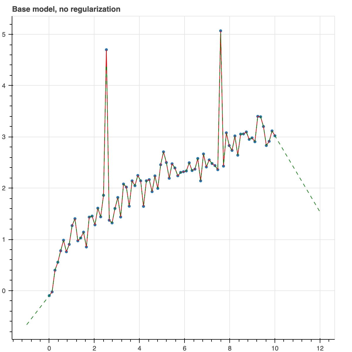
This has no real use by itself. It's just saying the model is the same as the data points.
You'll always want to give it some key-words to apply some kind of regularization or constraint so that the model is not simply the same as the noisy data.
Let's do something more useful. Don't do any regularization yet. Just force the model to be monotonically increasing. So basically, it is looking for the model which has minimal Huber loss but is constrained to be monotonically increasing.
We use Huber loss because it is robust to outliers while still looking like quadratic loss for small values.
result = trend_filter(x, y_noisy, monotonic=True)
plot_model(result, show_extrap=True, extrap_max=3)
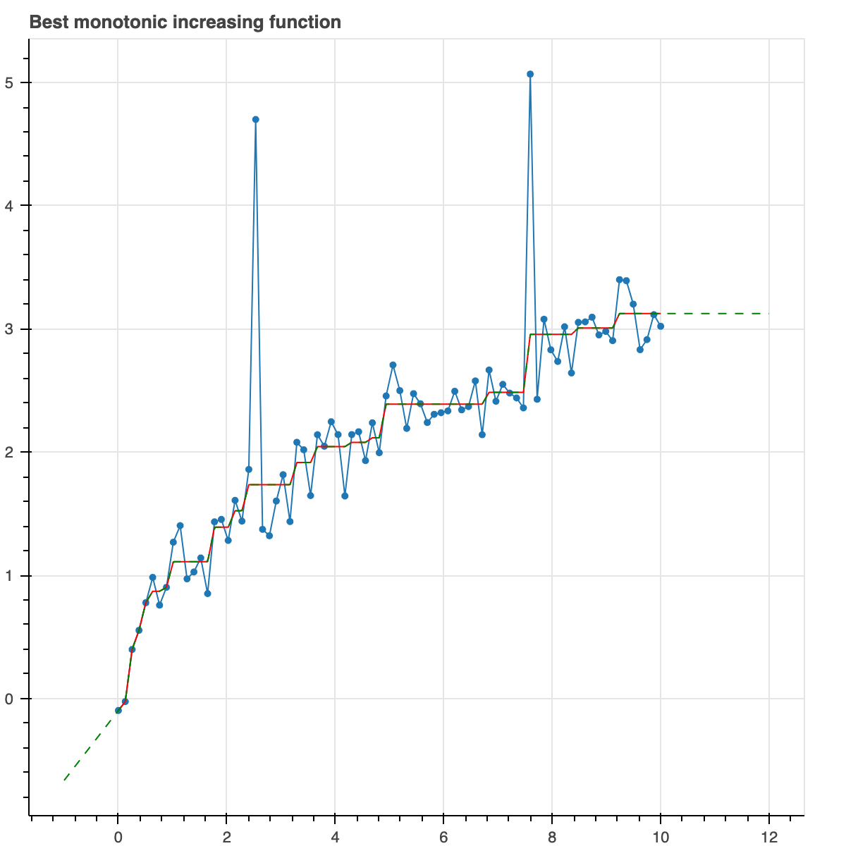
The green line, by the way, just shows that the function can be extrapolated which is a very useful thing, for example, if you want to make predictions about the future.
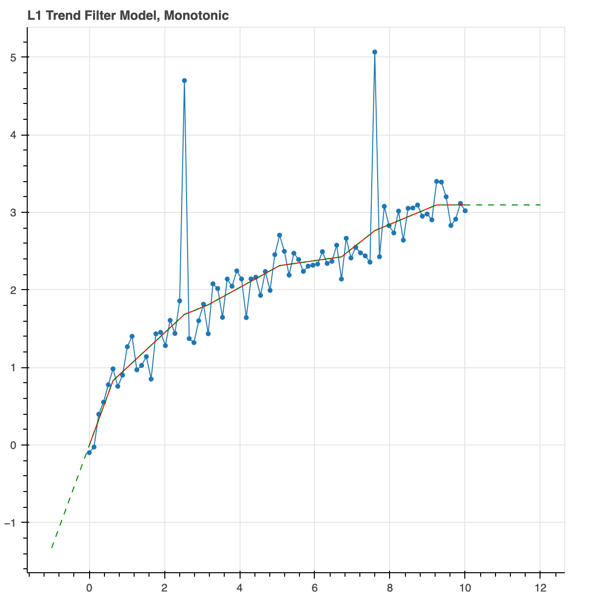
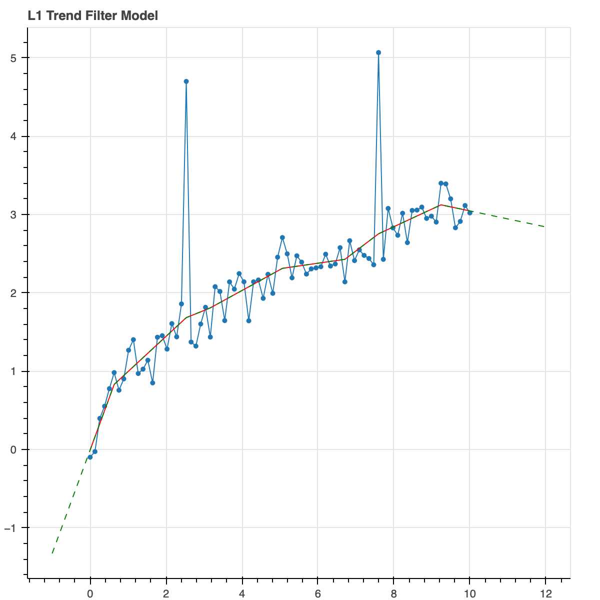
Ok, now let's do an L1 trend filter model. So we are going to penalize any non-zero second derivative with an L1 norm. As we probably know, L1 norms induce sparseness. So the second dervative at most of the points will be exactly zero but will probably be non-zero at a few of them. Thus, we expect piecewise linear trends that occasionally have sudden slope changes.
result = trend_filter(x, y_noisy, l_norm=1, alpha_2=0.2)
plot_model(result, show_extrap=True, extrap_max=3)
Let's do the same thing but enforce it to be monotonic.
result = trend_filter(x, y_noisy, l_norm=1, alpha_2=0.2, monotonic=True)
plot_model(result, show_extrap=True, extrap_max=3)
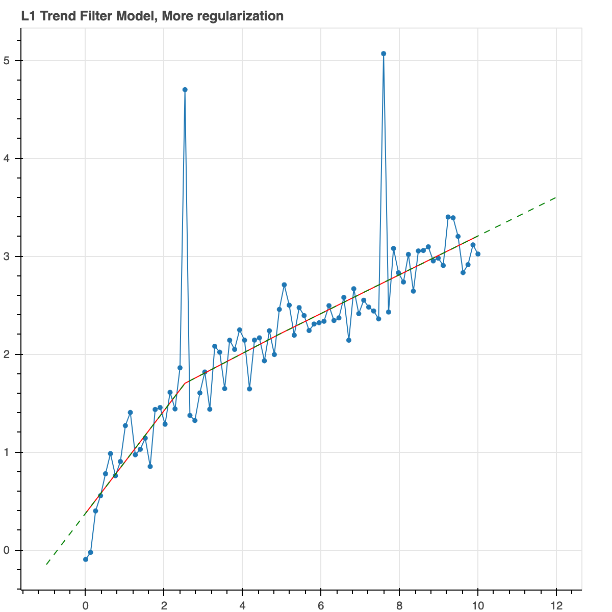
Now let's increase the regularization parameter to give a higher penalty to slope changes. It results in longer trends. Fewer slope changes. Overall, less complexity.
result = trend_filter(x, y_noisy, l_norm=1, alpha_2=2.0)
plot_model(result, show_extrap=True, extrap_max=3)
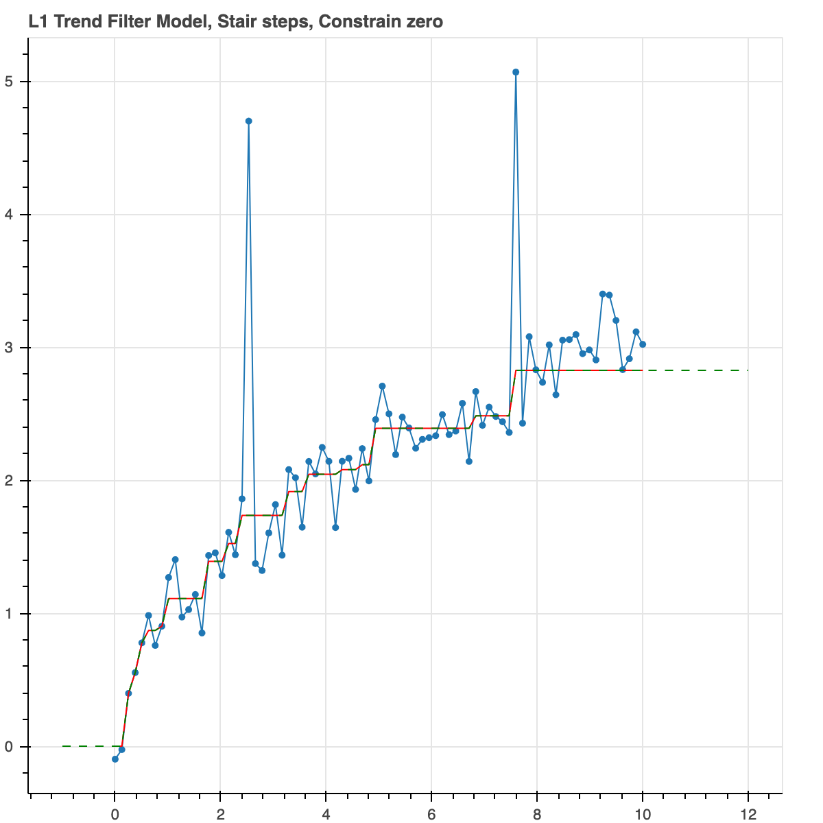
Did you like the stair steps? Let's do that again. But now we will not force it to be monotonic. We are going to put an L1 norm on the first derivative. This produces a similar output but it could actually decrease if the data actually did so. Let's also constrain the curve to go through the origin, (0,0).
result = trend_filter(x, y_noisy, l_norm=1, alpha_1=1.0, constrain_zero=True)
plot_model(result, show_extrap=True, extrap_max=3)
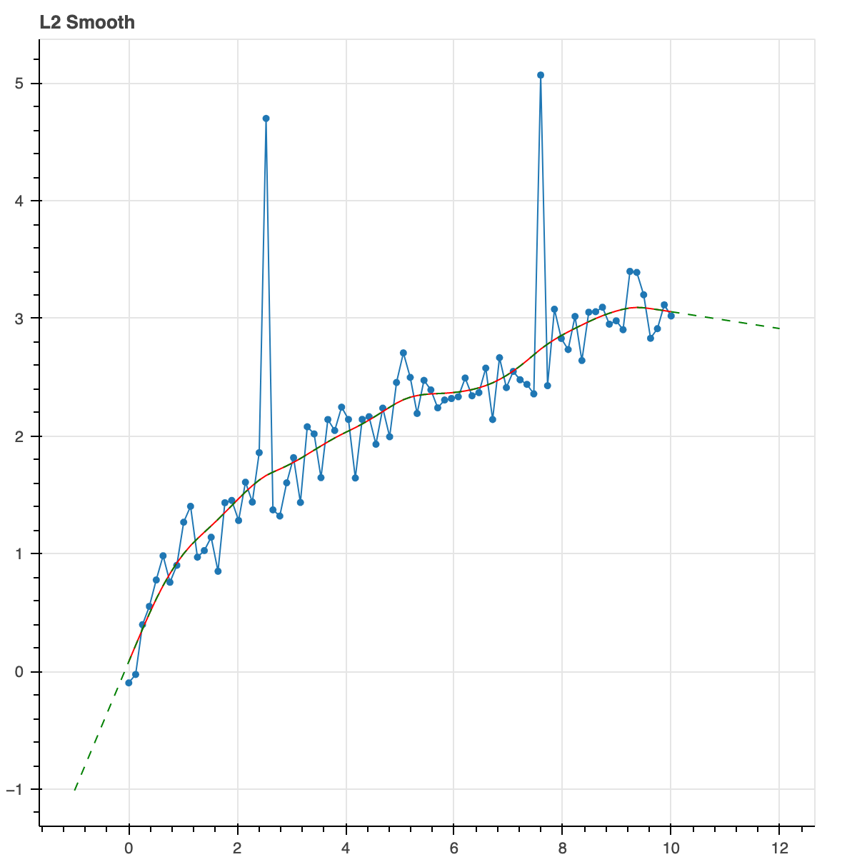
Let's do L2 norms for regularization on the second derivative. L2 norms don't care very much about small values. They don't force them all the way to zero to create sparse solution. They care more about big values. This results is a smooth continuous curve. This is a nice way of doing robust smoothing.
result = trend_filter(x, y_noisy, l_norm=2, alpha_2=2.0)
plot_model(result, show_extrap=True, extrap_max=3)
Here is the full function signature.
def trend_filter(x, y, y_err=None, alpha_1=0.0,
                 alpha_2=0.0, l_norm=2,
                 constrain_zero=False, monotonic=False,
                 positive=False,
                 linear_deviations=None):
So you see there are alpha key-words for regularization parameters. The number n, tells you the derivative is being penalized. You can use any, all or none of them. The key-word l_norm gives you the choice of 1 or 2. Monotonic and constrain_zero, we've explained already. positive forces the base model to be positive. linear_deviations will be explained in a bit.
The data structure returned by trend_filter is a dictionary with various pieces of information about the model. The most import are 'y_fit' which is an array of best fit model values corresponding to each point x. The 'function' element is a function mapping any x to the model value, including points outside the initial range. These external points will be extrapolated linearly. In the case that the data is a time-series, this function can provide forecasts for the future.
We didn't discuss y_err. That's the uncertainty on y. The default is 1. The Huber loss is actually applied to (data-model)/y_err. So, you can weight points differently if you have a good reason to, such as knowing the actual error values or knowing that some points are dubious or if some points are known exactly. That would be the limit as y_err goes towards zero and it will make the curve go through those points.
All in all, these keywords give you a huge amount of freedom in what you want your model to look like.
Linear model deviations and seasonality:
Any time series library should include ways of modeling seasonality and this one does as well. In fact, it includes something more general which is the ability to add in any linear features to the model. This linearity preserves convexity and so we can still use convex optimization. By linear deviation we means any addition to the model that is a specified matrix multiplied by a variable vector. That variable vector can be solved for as well.
To do this you create a data structure called linear deviations
linear_deviation = {'mapping': lambda x: int(x) % 12,
                    'name': 'seasonal_term',
                    'n_vars': 12,
                    'alpha': 0.1}
This assumes the matrix above is an assignment matrix. You can also create a matrix yourself and include that as 'matrix' instead of 'mapping'.
This provides a mapping from x to some set of integer indices. You tell it there are 12 of them. One for each month of the year. We can give it a name 'seasonal_term' and a regularization parameter. Evidently, we are going to use this on a monthly time series.
Now just call it like this.
linear_deviations = [linear_deviation]
result = trend_filter(x, y_noisy, l_norm=1, alpha_2=4.0, linear_deviations=linear_deviations)
Note that you input it as a list if linear deviations. You can include multiple. Perhaps for example, you have one that marks months for which the kids are in school or months where there was a convention in town.
Let's see it in action.
We've created another data set with some seasonal pattern added. This is how it looks when the model is run without seasonality.
from trendfilter import get_example_data_seasonal()

x, y_noisy = get_example_data_seasonal()
result = trend_filter(x, y_noisy,  l_norm=1, alpha_2=4.0)
plot_model(result, show_extrap=True, extrap_max=40)
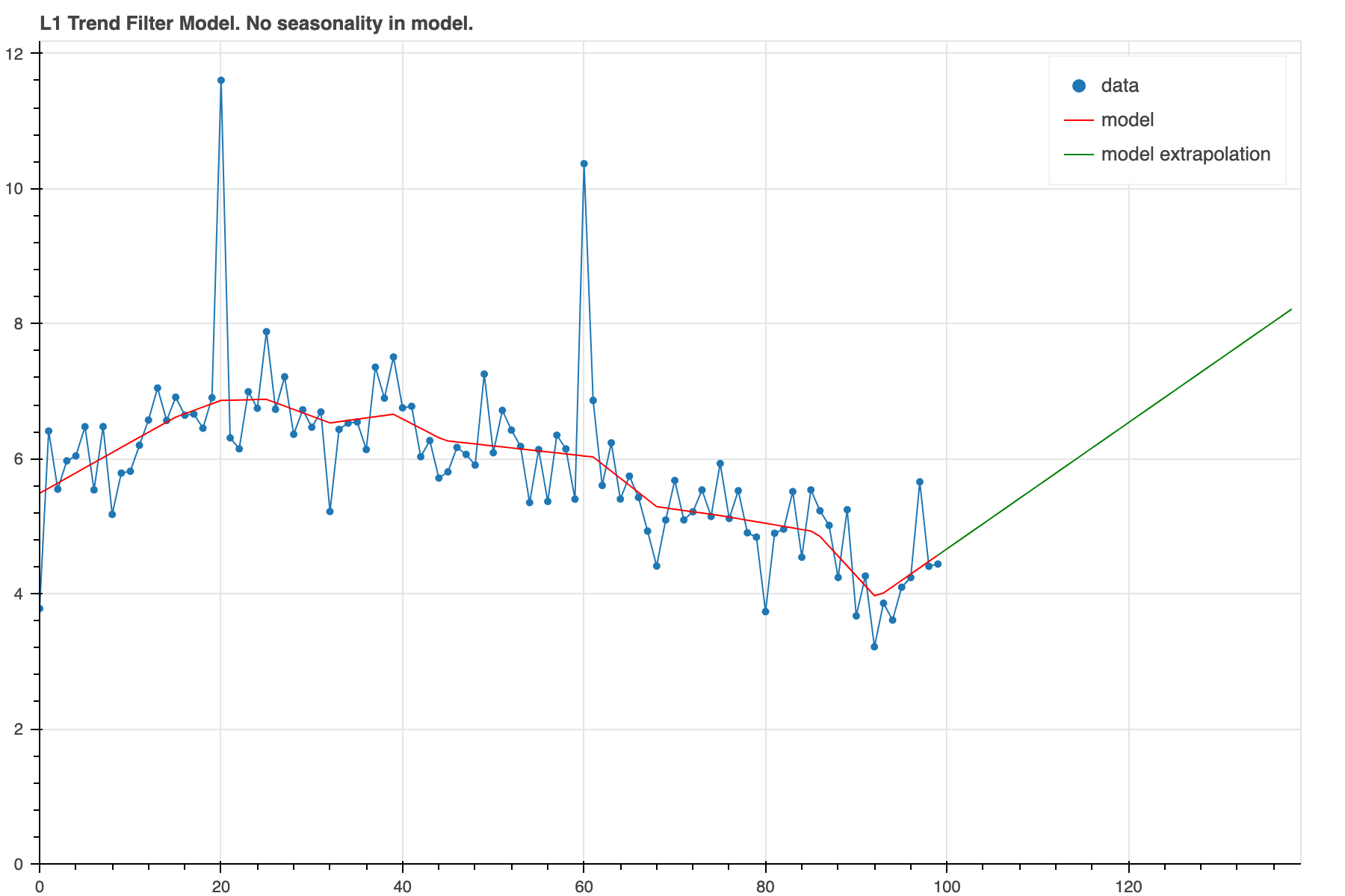
In this case the model is just trying to model all the wiggles with a changing trend. This doesn't produce a very convincing looking forecast. We can improve that some and iron out the wiggles by using a higher alpha_2.
But if we notice there is some periodicity to it, we can actually model it using the structure we created above.
result = trend_filter(x, y_noisy, l_norm=1, alpha_2=4.0, linear_deviations=linear_deviations)
plot_model(result, show_extrap=True, extrap_max=40, show_base=True)
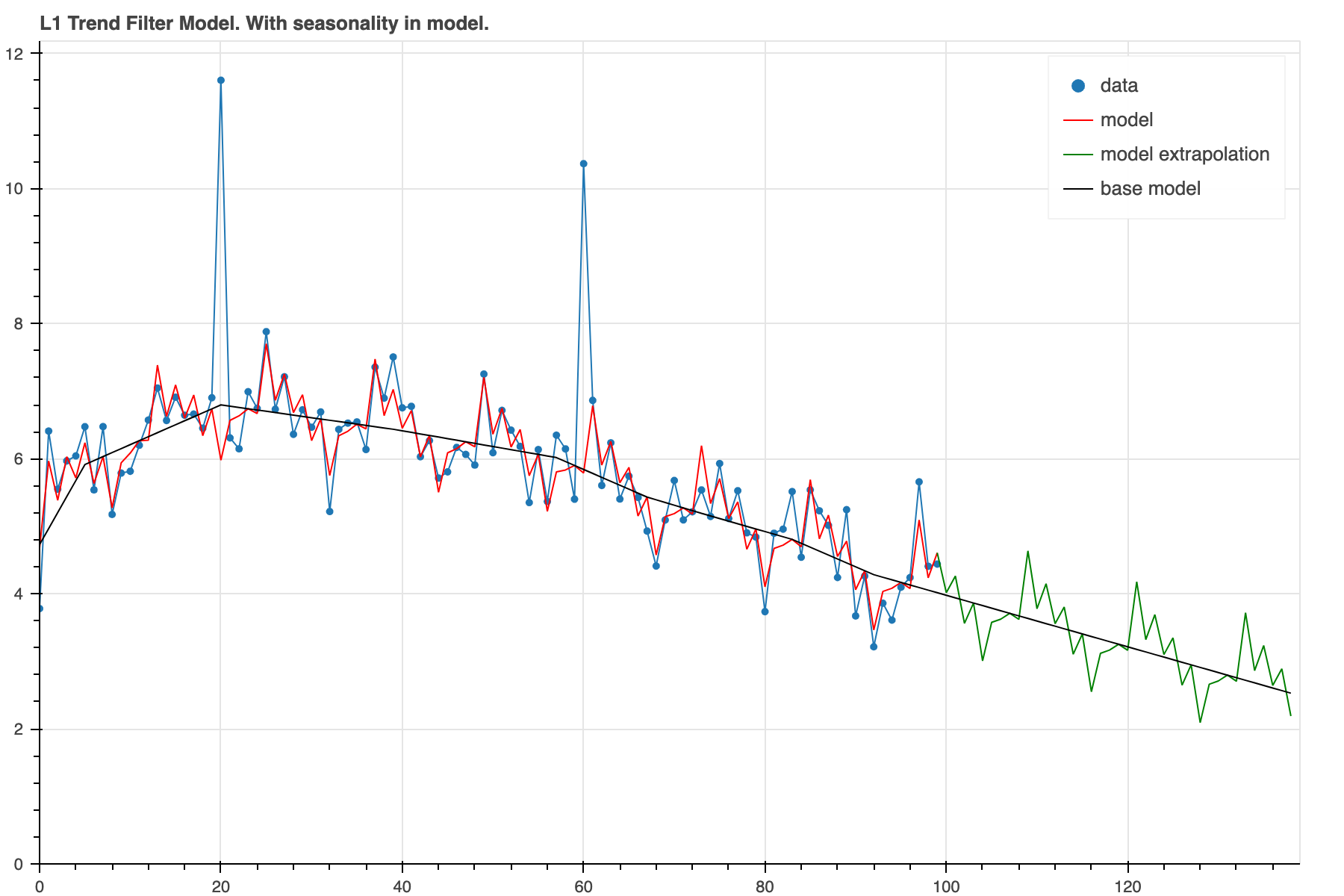
Now, we can see that there is indeed a prominant seasonal pattern on top of a rather smooth base model. The forecast now will include that same seasonal pattern which should lead to a more accurate forecast.
The 'alpha' regularization determines the amount of evidence required to make use of the seasonal component. For a larger alpha and the same pattern here, it will take more cycles before it will overcome the barrier. At this point the total objective is lower than trying to model the wiggles with slope changes or tolerating a difference between model and data.
First pypi version April 12, 2021
0.1.4 Added more examples with more documentation and plots in the Readme
0.1.5 Mostly a refactor but changed API slightly.
0.2.0 Includes seasonality and linear deviations.
0.2.1 Switched to ECOS solver
0.3.0 Switched to Claribel solver which is the new built in solver Inputs now converted to numpy arrays so list inputs should work
0.3.2 Fixing PyPi to show plots, use full URLs
Release history Release notifications | RSS feed


Download files
Download the file for your platform. If you're not sure which to choose, learn more about installing packages.
Source Distribution
Built Distribution
Filter files by name, interpreter, ABI, and platform.
If you're not sure about the file name format, learn more about wheel file names.
Copy a direct link to the current filters
File details
Details for the file trendfilter-0.3.2.tar.gz.
File metadata
- Download URL: trendfilter-0.3.2.tar.gz
- Upload date:
- Size: 16.0 kB
- Tags: Source
- Uploaded using Trusted Publishing? No
- Uploaded via: twine/5.1.1 CPython/3.9.6
File hashes
| Algorithm | Hash digest | |
|---|---|---|
| SHA256 |
91b21d9767f63aa3d4767e910d2ae8eff5562379fcad659a8022595b0de29eed
|
|
| MD5 |
45af0ccdfa5d3e3013975cf5ab0ccb22
|
|
| BLAKE2b-256 |
8ca346b22c6f81de6afb14f44ac454e06edc74a6d876930c970a3290c54b8f1b
|
File details
Details for the file trendfilter-0.3.2-py3-none-any.whl.
File metadata
- Download URL: trendfilter-0.3.2-py3-none-any.whl
- Upload date:
- Size: 13.0 kB
- Tags: Python 3
- Uploaded using Trusted Publishing? No
- Uploaded via: twine/5.1.1 CPython/3.9.6
File hashes
| Algorithm | Hash digest | |
|---|---|---|
| SHA256 |
a56bffd2f8852f272384bf32c1b8fe00154d95ed7965d226359e9a981a332548
|
|
| MD5 |
2875a88b4083cb9840f2f4c7b46c6f65
|
|
| BLAKE2b-256 |
370a463337a8dfae672d718959701d748ed431e5345b63e33927c194811711c6
|


