
Time Series Analysis with Python
This is the collection of notebooks for the course Time Series Analysis with Python. You can view and execute the notebooks by clicking on the buttons below.
📑 Content
-
Introduction to time series analysis
- Definition of time series data
- Main applications of time series analysis
- Statistical vs dynamical models perspective
- Components of a time series
- Additive vs multiplicative models
- Time series decomposition techniques
or

-
Stationarity in time series
- Stationarity in time series
- Weak vs strong stationarity
- Autocorrelation and autocovariance
- Common stationary and nonstationary time series
- How to identify stationarity
- Transformations to achieve stationarity
-
Smoothing
- Smoothing in time series data
- The mean squared error
- Simple average, moving average, and weighted moving average
- Single, double, and triple exponential smoothing
-
AR-MA
- The autocorrelation function
- The partial autocorrelation function
- The Auto-Regressive model
- The Moving-Average model
- Reverting stationarity transformations in forecasting
-
ARMA, ARIMA, SARIMA
- Autoregressive Moving Average (ARMA) models
- Autoregressive Integrated Moving Average (ARIMA) models
- SARIMA models (ARIMA model for data with seasonality)
- Automatic model selection with AutoARIMA
- Model selection with exploratory data analysis
-
Unit root test and Hurst exponent
- Unit root test
- Mean Reversion
- The Hurst exponent
- Geometric Brownian Motion
- Applications in quantitative finance
-
Kalman filter
- Introduction to Kalman Filter
- Model components and assumptions
- The Kalman Filter algorithm
- Application to static and dynamic one-dimensional data
- Application to higher-dimensional data
-
Signal transforms and filters
- Introduction to Fourier Transform, Discrete Fourier Transform, and FFT
- Fourier Transform of common signals
- Properties of the Fourier Transform
- Signal filtering with low-pass, high-pass, band-pass, and bass-stop filters
- Application of Fourier Transform to time series forecasting
-
Prophet
- Introduction to Prophet for time series forecasting
- Advanced modeling of trend, seasonality, and holidays components
- The Prophet library in Python
-
Neural networks and Reservoir Computing
- Windowed approaches and Neural Networks for time series forecasting
- Forecasting with a Multi-Layer Perceptron
- Recurrent Neural Networks: advantages and challenges
- Reservoir Computing and the Echo State Network
- Dimensionality reduction with Principal Component Analysis
- Forecasting electricity consumption with Multi-Layer Perceptron and Echo State Network
-
Non-linear time series analysis
- Dynamical systems and nonlinear dynamics
- Bifurcation diagrams
- Chaotic systems
- High-dimensional continuous-time systems
- Fractal dimensions
- Phase space reconstruction and Taken's embedding theorem
- Forecasting time series from nonlinear systems
-
Time series classification and clustering
- Multivariate time series
- Time series similarities and dissimilarities
- Dynamic Time Warping
- Time series kernels
- Embedding time series into vectors
- Classification of time series
- Clustering of time series
- Visualize time series with kernel PCA
💻 How to code locally
To run the notebooks locally the recommended steps are the following:
-
Download and install Miniconda.
-
Download the env.yml file.
-
Open the shell and navigate to the location with the
ymlfile you just downloaded.- If you are on Windows, open the Miniconda shell.
-
Install the environment with
> conda env create -f env.yml
-
Activate your environment:
> conda activate pytsa
-
Go to the folder with the notebooks
-
Launch Jupyter Lab with the command
> jupyter lab
🎥 Notebook format and slides
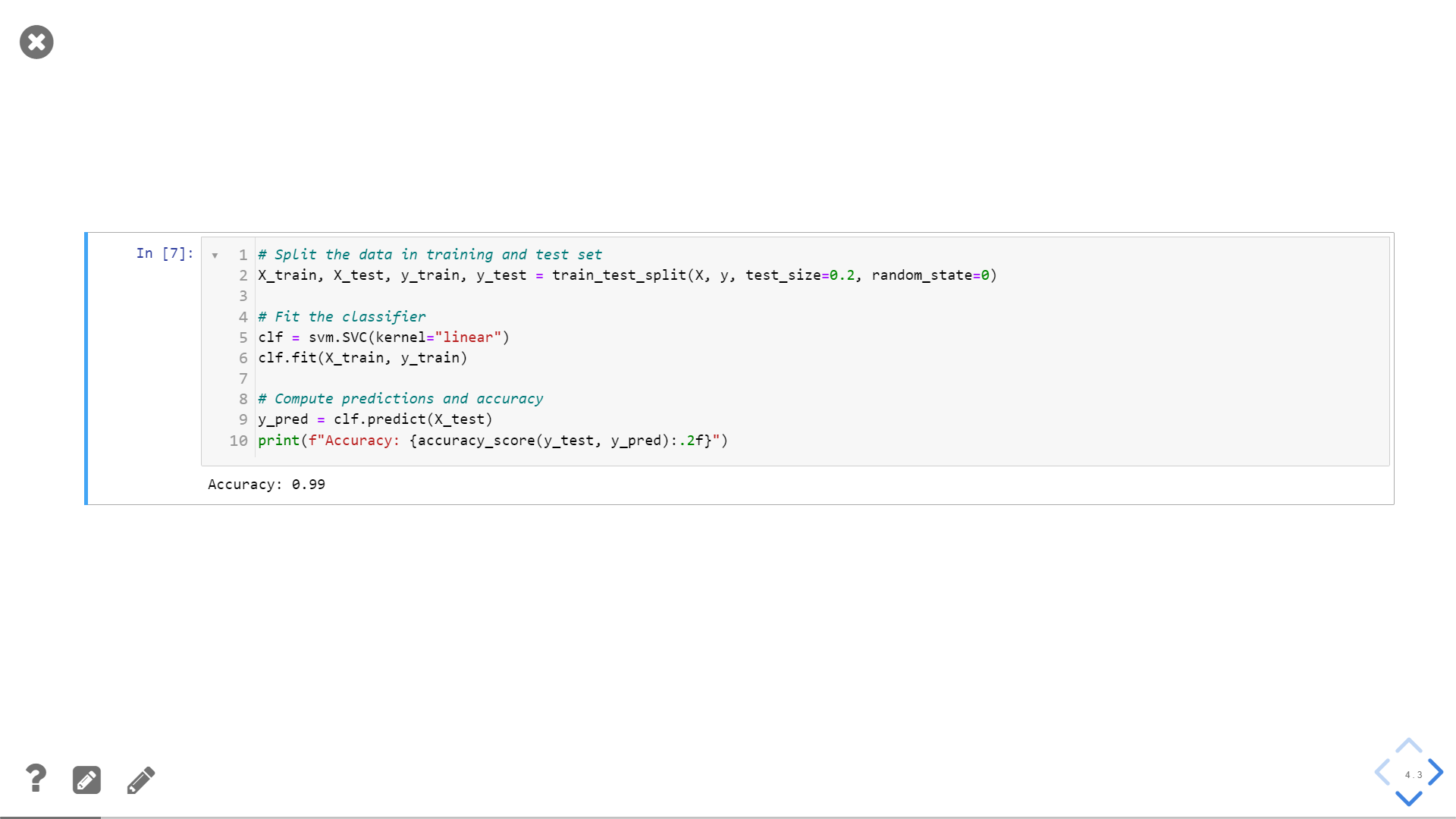
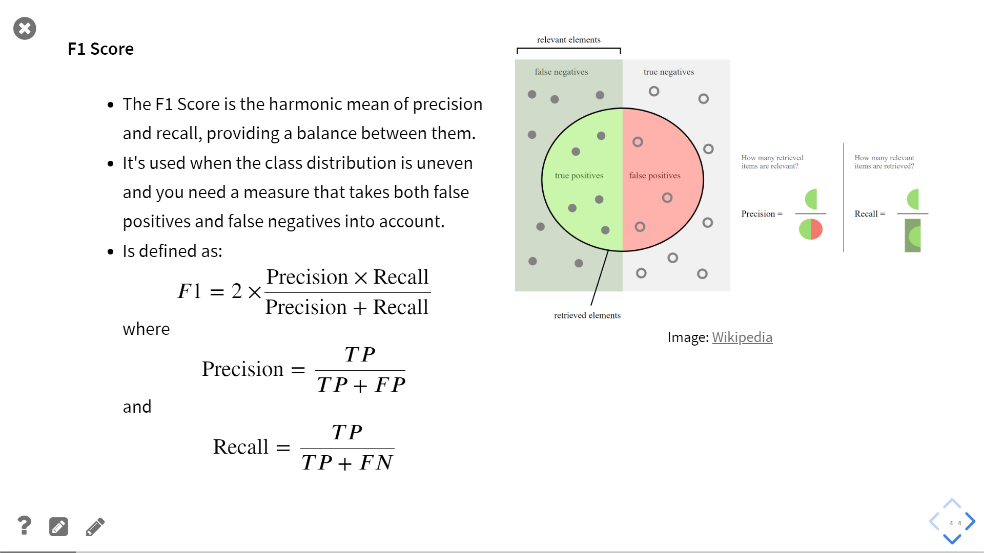
The notebooks are structured as a sequence of slides to be presented using RISE. If you open a notebook you will see the following structure:
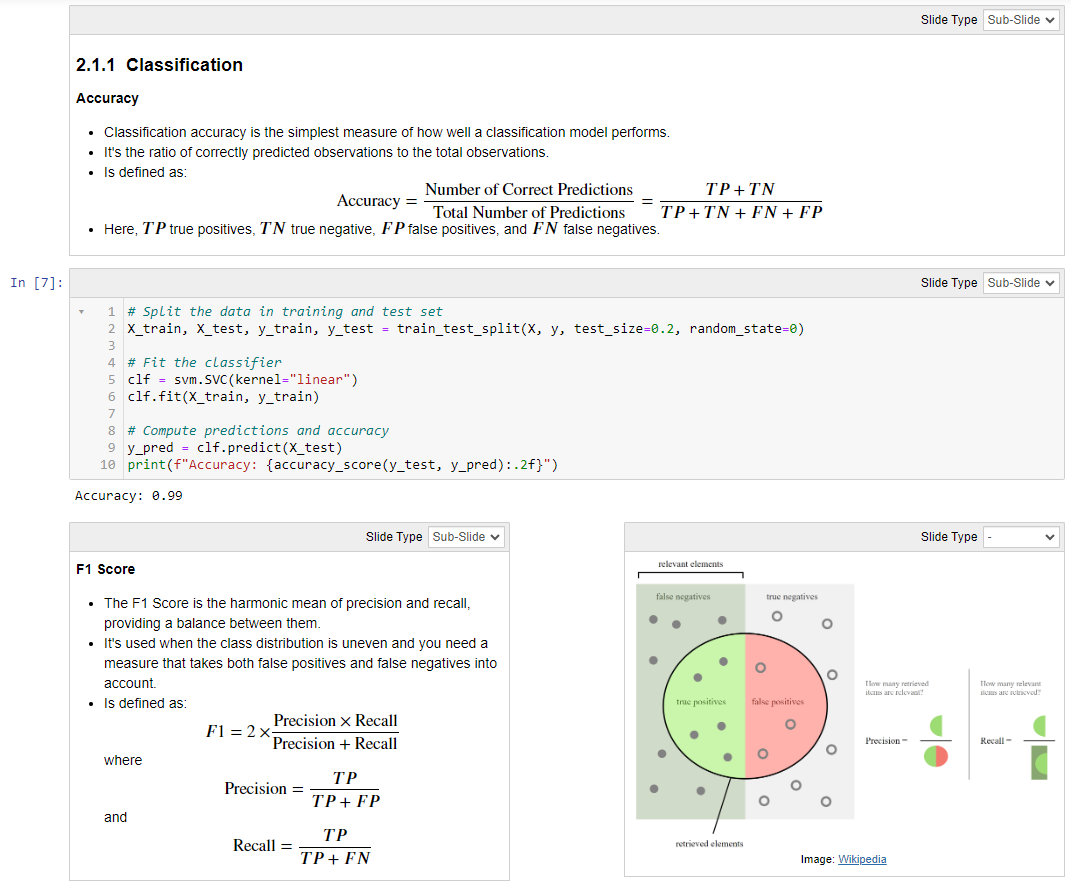
The top-right button indicates the type of slide, which is stored in the metadata of the cell. To enable the visualization of the slide type you must first install RISE and then on the top menu select View -> Cell Toolbar -> Slieshow. Also, to split the cells like in the example, you must enable Split Cells Notebook from the nbextensions.
By pressing the Enter\Exit RISE Slideshow button at the top you can enter the slideshow presentation.
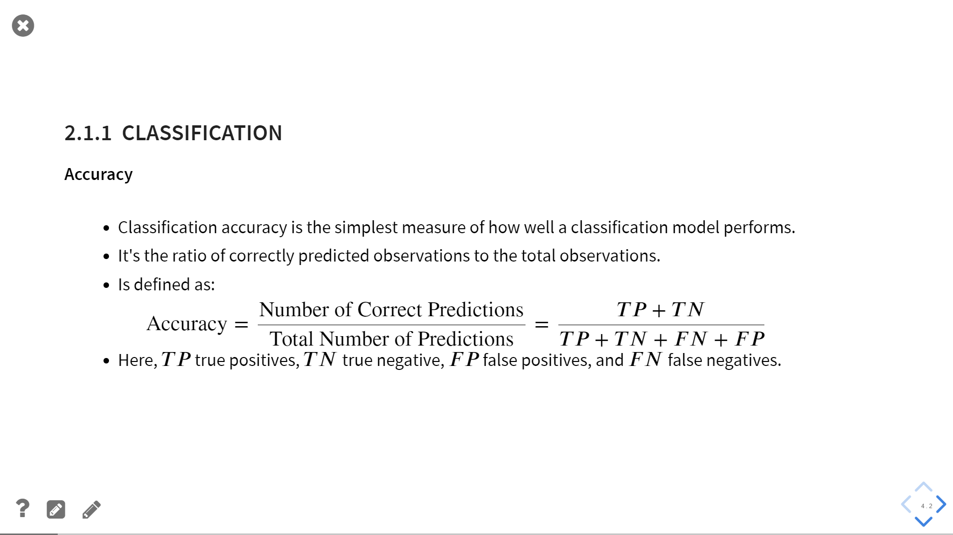
See the RISE documentation for more info.
📝 Citation
If you are using this material in your courses or in your research, please consider citing it as follows:
@misc{bianchi2024tsbook,
  author       = {Filippo Maria Bianchi},
  title        = {Time Series Analysis with Python},
  year         = {2024},
  howpublished = {Online},
  url          = {https://github.com/FilippoMB/python-time-series-handbook}
}
1 maintainer

Metadata
1 maintainer
Release files for tsa-course 0.3.1
For a detailed explanation of source distributions (sdists) and built distributions (wheels), please see the package formats documentation.
Source distribution (sdist)
| File | Size | Uploaded | |
|---|---|---|---|
| tsa_course-0.3.1.tar.gz | 13.4 kB | Details |
Built distribution (wheel)
| File | Interpreter | ABI | Platform | Reset |
|---|---|---|---|---|
| tsa_course-0.3.1-py3-none-any.whl | Python 3 | none | any | Details |
Total release size: 24.6 kB
Release files / tsa_course-0.3.1.tar.gz
| Download URL | tsa_course-0.3.1.tar.gz |
|---|---|
| Size | 13.4 kB |
| Tags | Source |
|
SHA-256 checksum How to use checksums |
b1496e29b8b5679ea77cc10759b139012102d159d1684ebd4a162386adda1782
|
|
BLAKE2b-256 checksum How to use checksums |
bfebb87872d03724793a245b75c7e886674106850d40d8f1987fc8acd5492e4f
|
| Upload date | |
|
Uploaded using Trusted Publishing? What is trusted publishing? |
No |
| Uploaded via |
twine/6.1.0 CPython/3.10.16
|
Release files / tsa_course-0.3.1-py3-none-any.whl
| Download URL | tsa_course-0.3.1-py3-none-any.whl |
|---|---|
| Size | 11.2 kB |
| Tags | Python 3 |
|
SHA-256 checksum How to use checksums |
f5c99bd4c37a13623a4a4939a6dec6b43e7fb96c6103b74fbcee995a50b4e9ab
|
|
BLAKE2b-256 checksum How to use checksums |
060d079bc97b5bd5569ae9d3f511baef91209542a4a4afc94ff6eac5d9e2bde1
|
| Upload date | |
|
Uploaded using Trusted Publishing? What is trusted publishing? |
No |
| Uploaded via |
twine/6.1.0 CPython/3.10.16
|














