
tsdml — Double Machine Learning for Time Series



A complete, faithful Python implementation of
Ciganovic, M., D'Amario, F. and Tancioni, M. (2026). Double Machine Learning for Time Series. The Econometrics Journal. arXiv:2603.10999
Standard Double Machine Learning (Chernozhukov et al., 2018) needs randomised cross-fitting, which shreds the sequential structure of a time series. The existing fix — Neighbors-Left-Out cross-fitting — deletes buffer blocks around each fold, which is expensive when you only have 60 quarters of data.
tsdml implements the paper's two answers:
| What it does | Why it matters | |
|---|---|---|
| Reverse Cross-Fitting | Trains nuisances on time-reversed auxiliary blocks and deletes no buffer | Uses 67% of the sample at K=6 where NLO uses 56% |
| Goldilocks-zone tuning | Picks the penalty inside a locally stable region of the validation-error profile, not at its global minimum | Predictive tuning over-shrinks the policy equation; this cuts small-sample bias by ~24% |
Plus everything around them: DML local projections for impulse responses, HAC inference with five bandwidth rules and fixed-b critical values, the conditional-stability diagnostic, and journal-ready figures and LaTeX tables.
Every number in this package has been verified bit-for-bit against the authors' own replication code, from data preparation through to the scaled impulse responses of Figure 2. See Fidelity.
📘 Documentation
➡️ Read the full step-by-step guide
A thirteen-step, annotated walkthrough that writes the code with you — from a raw CSV to a submitted figure. Every argument explained, every choice justified, with a troubleshooting section at the end.
| Document | What it covers |
|---|---|
| Step-by-step guide | The complete tutorial: shape your data → choose K → tune → estimate → diagnose → impulse responses → figures → tables → robustness |
| Quickstart script | The five-step workflow in ~80 lines, runnable |
| Empirical replication | The paper's Section 5 application end to end |
| Method comparison | Monte Carlo: Goldilocks vs RMSE, RCF vs NLO |
| Changelog | What is in each release |
| Data sources | Provenance of the bundled dataset |
In Python, every object carries full numpydoc documentation with runnable examples:
help(tsdml.ReverseCrossFitting)
help(tsdml.Calibrator)
Contents
- Documentation
- Install
- 60-second example
- The method in five minutes
- Step-by-step guide
- Working with your own data
- Local projections
- Figures
- Tables
- Diagnostics: do not skip this
- Choosing K
- HAC inference
- The bundled dataset
- API reference
- Fidelity
- Known limits
- Citation
Install
pip install tsdml
From source:
git clone https://github.com/merwanroudane/tsdml.git
cd tsdml
pip install -e ".[dev]"
pytest
Requires Python ≥ 3.9. Dependencies (numpy, pandas, scipy,
scikit-learn, statsmodels, matplotlib, joblib) all install
automatically — there is nothing to compile and no R or Stata involved.
Check it works:
python -c "import tsdml; print(tsdml.__version__); print(tsdml.sample_use_table([6,11,12]))"
60-second example
import numpy as np
from sklearn.linear_model import Lasso
from tsdml import Calibrator, ReverseCrossFitting, simulate_plr

sim = simulate_plr(T=200, p=100, theta=1.5, seed=0)
X, y, d = sim["X"], sim["y"], sim["d"]           # time-ordered!

grid = {"alpha": np.linspace(1e-6, 0.4, 100), "max_iter": [100_000]}

cal = Calibrator(metric="goldilocks_zone", n_blocks=6)
cal.calibrate(X, y, d,
              outcome_learner_class=Lasso,    outcome_param_grid=grid,
              treatment_learner_class=Lasso,  treatment_param_grid=grid)

model = ReverseCrossFitting(
    n_blocks=6,
    block_specific_learners=cal.block_specific_learners_,
).fit(X, y, d)

model.summary()
========================================================================
Reverse Cross-Fitting DML  --  partially linear model
========================================================================
observations         : 200
folds (K)            : 6   block size 33
stage-2 method       : block
HAC                  : bartlett (rule 'small')
------------------------------------------------------------------------
                    coef     std err         t     P>|t|
theta           1.367399    0.083104    16.450    0.0000 ***
95% CI: [1.204518, 1.530280]
fold estimates: [1.0824, 1.0374, 1.6421, 1.4585, 1.3540, 1.6300]
========================================================================
The method in five minutes
The model
A partially linear model with a scalar policy variable and possibly many controls (paper, eqs. 1.1–1.2):
y_t = θ₀ d_t + g₀(X_t) + ε_t ,      E[ε_t | X_t, d_t] = 0
d_t =        m₀(X_t) + ξ_t ,        E[ξ_t | X_t]      = 0
θ₀ is what you want. g₀ and m₀ are nuisances you must estimate well enough
that their error does not contaminate θ̂ — that is what orthogonalisation plus
cross-fitting buys you.
Reverse Cross-Fitting
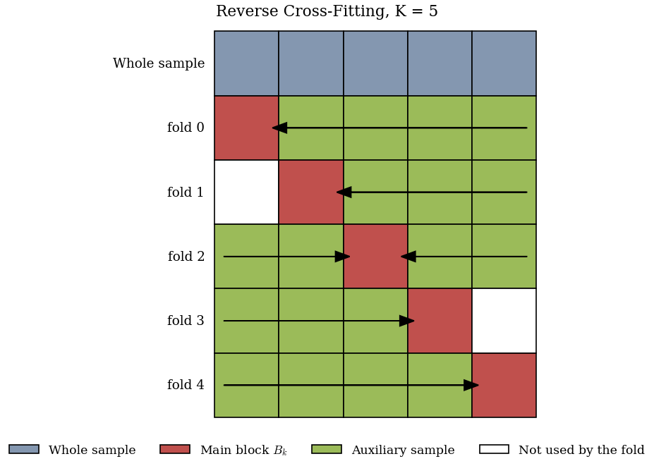
Cut the sample into K adjacent blocks B₁ … B_K. For fold k:
    ┌───────┬───────┬───────┬───────┬───────┐
k=0 │ MAIN  │  aux  │  aux  │  aux  │  aux  │  ← train right, read time BACKWARDS
    ├───────┼───────┼───────┼───────┼───────┤
k=1 │   ·   │ MAIN  │  aux  │  aux  │  aux  │  ← train right, backwards
    ├───────┼───────┼───────┼───────┼───────┤
k=2 │  aux  │  aux  │ MAIN  │  aux  │  aux  │  ← both sides, average (odd K only)
    ├───────┼───────┼───────┼───────┼───────┤
k=3 │  aux  │  aux  │  aux  │ MAIN  │   ·   │  ← train left, forward
    ├───────┼───────┼───────┼───────┼───────┤
k=4 │  aux  │  aux  │  aux  │  aux  │ MAIN  │  ← train left, forward
    └───────┴───────┴───────┴───────┴───────┘
Two things are doing work here.
Time reversibility. Stationary Gaussian processes have the same finite-dimensional distributions read forwards or backwards, so a nuisance fitted on the reversed right-hand blocks targets the same population function as one fitted forwards. That licences using the future as training data for the past.
No buffer. Unlike NLO, nothing is deleted between the auxiliary and main samples. Validity comes instead from conditional stability (Assumption 2.4):
E[ξ_t | X_t, F_aux,k] = 0 and E[ε_t | X_t, F_aux,k] = 0
After conditioning on X_t, the adjacent training blocks must carry no
information about the main-block innovations. Reversibility does not imply
this, and it does not imply reversibility — they are separate requirements.
tsdml gives you a test for it (see Diagnostics).
Estimation is then residual-on-residual OLS within each main block, averaged across folds (eq. 2.5), with HAC inference built from the stacked, time-ordered score sequence so that dependence across block boundaries is picked up.
The Goldilocks zone
The penalty that minimises prediction error is not the penalty that minimises bias in the causal score. Over-shrink the policy equation and you attenuate the partialled-out signal; under-shrink and you absorb policy variation into the controls. The paper's rule targets a locally stable region instead:
For each window W_j of S consecutive grid points:
    R̄_j = mean RMSE in the window          (level)
    V_j  = variance of RMSE in the window   (stability)
    S_j  = normalise(V_j) + normalise(R̄_j)

j* = argmin S_j                             pick the most stable good window
λ* = argmin RMSE within W_j*                then the best point inside it
Default S = 3. plot_goldilocks_profile shows you the picture:
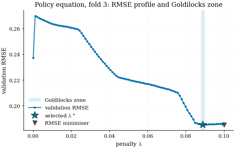
The star is λ*; the grey triangle is the plain RMSE minimiser. When they diverge, the rule is doing something.
Step-by-step guide
A complete, annotated walkthrough — from a raw CSV to a submitted figure — is
in docs/STEP_BY_STEP_GUIDE.md. It writes the
code with you, line by line, and explains the choice behind each argument.
Runnable scripts:
| Script | What it does | Runtime |
|---|---|---|
examples/01_quickstart.py |
The five-step workflow on simulated data, plus the conditional-stability check firing and not firing | ~30 s |
examples/02_empirical_replication.py |
The paper's full Section 5 application: five outcomes, Figure 2, LaTeX tables | ~2 min |
examples/03_tuning_and_design_comparison.py |
Monte Carlo: Goldilocks vs RMSE, RCF vs NLO | ~3 min |
Working with your own data
tsdml accepts plain arrays, so you can bypass the data layer entirely:
model = ReverseCrossFitting(outcome_learner, treatment_learner, n_blocks=6)
model.fit(X, y, d)     # X (T, p), y (T,), d (T,) -- rows in calendar order
The only hard requirement: rows must be consecutive time periods in order. The block structure is positional. Shuffle the rows and the estimator is meaningless — it will not warn you, because it cannot tell.
If you want the paper's data pipeline (transformations, fast/slow timing, lags,
leads, fold-divisible truncation), use DataProcessor. It expects a wide table
with two metadata rows on top:
sasdate |
GDP |
Spread |
Yield10y |
|---|---|---|---|
| speed | slow | slow | fast |
| Transform: | 5 | 2 | 2 |
| 2005-06-30 | 107.51 | 1.25 | 3.44 |
| 2005-09-30 | 108.09 | 1.28 | 3.51 |
speedimplements the block-recursive timing assumption of Section 5.2.fastvariables (prices, yields, spreads, FX) enter the control set contemporaneously — they plausibly reflect within-quarter information.slowvariables (GDP, employment, bank balance sheets) enter only with lags, which keeps you from conditioning on post-treatment mediators sitting on the transmission path.Transform:is the stationarity transformation, FRED-MD convention:
| Code | Transformation | Code | Transformation | |
|---|---|---|---|---|
| 1 | level | 8 | log Δ₁₂ (monthly YoY) | |
| 2 | first difference | 81 | log Δ₄ (quarterly YoY) | |
| 3 | second difference | 9 | series ÷ HP trend | |
| 4 | log | 10 / 101 | Δ₁₂ / Δ₄ | |
| 5 | 100 × Δlog | 11 / 111 | 100 × YoY growth | |
| 6 | Δ²log | 7 | 100 × growth rate |
Codes 5, 7, 11 and 111 are multiplied by 100, so a log-differenced response
reads directly as a percentage change. tsdml.TRANSFORM_CODES lists them all.
from tsdml import DataProcessor

proc = DataProcessor()
X, y, d, leads = proc.data_prep(
    df=my_table,
    num_lags=3,                        # lags of every series, incl. y and d
    H=8,                               # horizons 0..8
    treatment_var="Policy rate", treatment_code=2,
    outcome_var="GDP",          outcome_code=5,
    start_date="2005-12-31",
    scaling_method="none",             # 'l2' | 'standard' | 'robust' | 'minmax'
    include_constant=True,
    K=6,                               # truncates so len(X) % K == 0
)
treatment_code and outcome_code must match the sheet's Transform: row
for those columns — they identify the transformed column, they do not override
it. You get a clear KeyError if they disagree.
Afterwards, proc.original_index holds the dates of the retained rows and
proc.feature_names_ the column names of X.
Local projections
Dynamic responses come from DMLLocalProjections, which residualises at every
horizon h = 0 … H and reuses the policy residuals across horizons (they do not
change, so stage one runs roughly half as often).
from tsdml import DMLLocalProjections

lp = DMLLocalProjections(
    block_specific_learners=cal.block_specific_learners_,
    n_blocks=6,
    outcome_code=5,          # <- drives cumulation, see below
    outcome_name="GDP",
)
lp.fit(X, y, d, leads, index=proc.original_index)

lp.summary()
irf = lp.to_frame()          # Horizon, Coefficient, Std_Error, CI_*_90, CI_*_95
outcome_code matters. For an outcome in differences, the level response is
the cumulative sum of the horizon-by-horizon effects. Passing the
transformation code makes tsdml do that for you, following eq. (5.18):
codes 2/3/5/7/9 cumulate, 8/10 cumulate and divide by 12, 81/101 cumulate and
divide by 4, None or 1 leaves the response uncumulated. Get this wrong and
your impulse response is a growth-rate path when you meant a level path.
To normalise several responses to a common shock:
from tsdml import scale_irfs

scaled = scale_irfs(
    {"Tier 1 capital": irf1, "Risk-weighted assets": irf2, "GDP": irf3, ...},
    numerator_var="Tier 1 capital",
    denominator_var="Risk-weighted assets",
    basis_point_vars=("Spread",),      # these get an extra ×100
    target_shock=0.5,                  # 50 basis points
)
Since the capital ratio is capital over risk-weighted assets, its impact
response is the difference of the two component responses; the scaling factor is
target / (θ̂₀ᶜᵃᵖ − θ̂₀ᴿᵂᴬ).
Figures
Every plotting function applies a journal style (serif, no top/right spine,
colourblind-safe Wong palette, editable PDF text) and returns the
matplotlib.Figure so you can keep editing.
from tsdml import plot_irf_panel

plot_irf_panel(
    scaled,
    order=["Tier 1 capital", "Risk-weighted assets", "PNFC_Spread",
           "PNFC_Lending_K2020", "GDP_K2020"],
    titles={"GDP_K2020": "GDP", ...},
    ylabels={"PNFC_Spread": "Basis points", ...},
    layout=(2, 3),
    highlight="GDP_K2020",
    save_path="figure2.pdf",
)
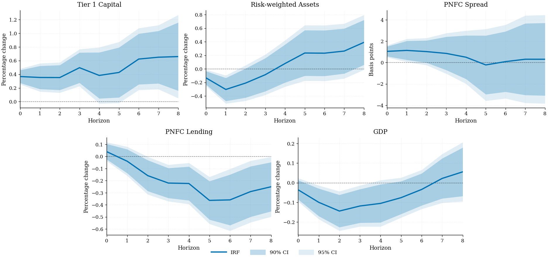
A ragged last row is centred at full panel width rather than stretched — pass
equal_widths=False for the stretched alternative.
| Function | Figure |
|---|---|
plot_irf |
one impulse response with nested 90/95% bands |
plot_irf_panel |
the multi-panel Figure 2 layout |
plot_irf_comparison |
several responses overlaid (Goldilocks vs RMSE, RCF vs NLO) |
plot_block_structure |
the fold diagram, Figure 1 |
plot_goldilocks_profile |
the RMSE profile, the selected window and λ* |
plot_sample_use |
RCF vs NLO sample use across K |
plot_residuals |
stage-one residuals with fold boundaries marked |
For slides: use_journal_style(serif=False, base_fontsize=13).
Tables
from tsdml import irf_table, estimation_table, calibration_table, to_latex

to_latex(
    irf_table(scaled["GDP_K2020"], digits=3),
    caption="Cumulative response of GDP to a 50bp rise in the Tier 1 ratio",
    label="tab:gdp",
    notes="RCF-DML local projections, Goldilocks-tuned Lasso, $K=6$. "
          "Newey-West standard errors in parentheses. "
          "*** $p<0.01$, ** $p<0.05$, * $p<0.10$.",
    save_path="table_gdp.tex",
)
Output is booktabs (needs \usepackage{booktabs}), with standard errors in
parentheses beneath each estimate and the usual significance stars.
to_markdown is there for READMEs and issue threads.
estimation_table puts several specifications side by side:
             RCF (Goldilocks)        RCF (RMSE)          NLO
theta               1.3674***         1.3641***    1.2988***
Std. error           (0.0831)          (0.0834)     (0.0952)
t-statistic            16.450            16.364       13.643
p-value                0.0000            0.0000       0.0000
95% CI       [1.2045, 1.5303]  [1.2007, 1.5275]  [1.112, 1.485]
Folds K                     6                 6            6
Sample use              0.667             0.667        0.556
Diagnostics: do not skip this
RCF buys its sample-use advantage by not deleting buffer blocks. The price is that conditional stability has to hold. It is an assumption about your data, not a property of the estimator, and it can fail — through residual serial dependence after conditioning, omitted persistent states, asymmetric volatility, or contemporaneously endogenous regimes.
from tsdml import diagnose

checks = diagnose(model)
print(checks["leakage_policy"])       # per fold and pooled
print(checks["ljungbox_outcome"])
boundary_leakage_test regresses main-block residuals on leads and lags drawn
from the adjacent blocks — precisely the observations a buffered design would
have thrown away — and joint-tests those coefficients. A small p-value says the
neighbours still predict the residuals.
It behaves as advertised. On simulate_plr with white-noise disturbances
(conditional stability holds) it rejects 0 times in 40 draws; give the
disturbances their own AR(1) dynamics (resid_persistence=0.7) and it rejects
29 times in 40, while coverage falls from 85% to 75%.
When it fires, in the order the paper suggests:
- Enrich
X_t— more lags, factor proxies, regime indicators — so the conditioning set absorbs the predictable component. This is the preferred fix when the problem is an omitted persistent state. - Switch to
NLOCrossFittingif the leakage is short-memory and will not go away. You buy independence and pay in sample use.
These are screening tools implementing a diagnostic the paper describes in words; they are not a line-by-line port of its supplementary appendix, and a rejection is a reason to think, not a formal test of Theorem 2.1.
Choosing K
K trades main-block size against auxiliary-sample size. The asymptotics hold
K fixed, so this is a finite-sample judgement.
from tsdml import sample_use_table
print(sample_use_table(range(3, 16)))
  K   u_RCF   u_NLO Winner
  3  0.6667  0.2222    RCF
  6  0.6667  0.5556    RCF
  9  0.7407  0.6914    RCF
 10  0.7000  0.7200    NLO
 11  0.7438  0.7438    tie
 12  0.7083  0.7639    NLO
RCF uses more of the sample than NLO for K = 3…9, they tie at K = 11, and
NLO wins at K = 10 and from K = 12 — so RCF is not uniformly better, it is
attractive in the moderate-K range where short macro samples live. The paper's
application uses K = 6, which gives a main-to-auxiliary ratio in line with
standard practice. Start there.
Two practical constraints: T // K must leave enough observations for a
stage-two regression in each block, and the Calibrator carves a validation
block of that same length out of the auxiliary sample, so very large K on a
short sample will raise a clear error rather than silently misbehave.
HAC inference
Theorem 2.1 needs a HAC estimate of the long-run variance of the stacked
score sequence — not an average of fold-wise variances. That is what
tsdml computes.
ReverseCrossFitting(
    ...,
    hac_kernel="bartlett",              # 'bartlett' | 'qs' | 'parzen' | 'ewc'
    hac_bandwidth_rule="small",         # see below
    use_fixed_b_critical=False,
)
| Rule | Bandwidth | Source |
|---|---|---|
'small' (default) |
min(h+1, 24) |
the paper's benchmark |
'newey-west' |
⌊4(T/100)^(2/9)⌋ |
Newey & West (1994) |
'andrews' |
AR(1) plug-in | Andrews (1991) |
'pow14' / 'pow15' |
⌊T^(1/4)⌋ / ⌊1.3221 T^(1/5)⌋ |
rules of thumb |
'lls_nw' |
⌈1.3 √T⌉ |
Lazarus, Lewis, Stock & Watson (2018) |
'lls_ewc' |
⌊0.4 T^(2/3)⌋ cosine terms |
LLSW (2018), EWC |
'fixed' |
hac_bandwidth_value |
yours |
use_fixed_b_critical=True switches to Kiefer–Vogelsang (2005) critical values
for Bartlett, or the exact Student-t fixed-b distribution for EWC. Pair it
with 'lls_nw' or 'lls_ewc' as LLSW recommend.
A caveat worth knowing. The default min(h+1, 24) is deliberately short.
When the cross-fitted score is strongly serially correlated it can produce
intervals that are too narrow — in a stress design with AR(0.8) disturbances,
observed coverage fell to about 75%. If your residual diagnostics show
persistence, move to 'lls_nw' with use_fixed_b_critical=True. The point
estimate is unaffected; only inference changes.
The bundled dataset
from tsdml import load_macroprudential, macroprudential_spec

df   = load_macroprudential()      # 37 series, 2005Q2-2024Q4, metadata rows on top
spec = macroprudential_spec()      # the paper's exact Section 5 specification
Quarterly Italian macro-financial and banking data assembled from official sources (IMF Financial Soundness Indicators, ISTAT, Bank of Italy, ECB and market data). The policy variable is the Tier 1 capital-to-risk-weighted-assets ratio; outcomes are Tier 1 capital, risk-weighted assets, the PNFC lending spread, PNFC lending and GDP.
macroprudential_spec() returns the treatment, outcomes and their codes, the
six variables dropped to avoid mechanical collinearity with the policy ratio,
num_lags=3, H=8, n_blocks=6, the start date, and plotting labels.
See src/tsdml/data/SOURCES.md for provenance and
redistribution notes.
API reference
Estimators
ReverseCrossFitting(outcome_learner, treatment_learner, n_blocks=5, ...)
    .fit(X, y, treatment, verbose=False) -> self
    .theta_, .results_, .residuals_, .blocks_
    .summary(), .to_frame(), .block_frame(), .plot_structure()

NLOCrossFitting(...)          # same interface, buffered design, K >= 4

DMLLocalProjections(..., outcome_code=None, n_blocks=6)
    .fit(X, y, treatment, leads, index=None) -> self
    .irf_, .results_, .estimators_
    .summary(), .to_frame(), .residuals_frame(), .plot(), .save(path)
Tuning
Calibrator(metric='goldilocks_zone', n_blocks=5, stability_window_size=3, n_jobs=1)
    .calibrate(X, y, treatment, outcome_learner_class=..., outcome_param_grid=..., ...)
    .block_specific_learners_, .rmse_profiles_, .calibration_scores_
    .summary(), .selected_params_frame()

goldilocks_select(rmse_profile, window_size=3) -> int
Folds and inference
reverse_cf_folds(n, K) -> BlockStructure
nlo_folds(n, K) -> (main, aux)
fold_direction(k, K) -> 'reverse' | 'both' | 'forward'
sample_use_rcf(K), sample_use_nlo(K)
hac_lrv(scores, K=0, kernel='bartlett', bandwidth=None)
compute_hac_bandwidth(rule, horizon=0, T=None, scores=None, value=None)
fixed_b_critical_value(kernel, b=None, nu=None, alpha=0.05)
fit_stage_two(chi, xi, estimation_method='block', ...)
Data
DataProcessor().data_prep(...) -> (X, y, policy, leads)
transform_series(x, tcode);  TRANSFORM_CODES
load_macroprudential();  macroprudential_spec()
simulate_svar(n, T, theta, specification='misspecified'|'specified', ...)
simulate_plr(T, p, theta, rho, resid_persistence=0.0, ...)
Diagnostics, figures, tables — listed in their sections above.
Everything is documented with numpydoc docstrings and runnable examples:
help(tsdml.ReverseCrossFitting).
Fidelity
The package was written against the authors' replication package and checked against it end to end on the paper's own data and specification:
| Checked | Result |
|---|---|
X, y, policy, leads from data_prep |
identical |
| Estimation index (dates, length 54) | identical |
| Stage-one residuals, both equations | identical |
| θ̂ and standard error, fixed-penalty RCF | identical to 1e-15 |
| Goldilocks-selected penalties, all 6 folds, both equations | identical |
| Impulse responses, all 5 outcomes, 9 horizons, 90% and 95% bands | identical |
| Scaled Figure 2 responses | identical |
Regression tests in tests/test_paper_replication.py
pin these values so they cannot drift, including the published GDP path
(−0.036, −0.100, −0.144 at h = 0, 1, 2) and the qualitative findings of
Section 5.3.
Run them:
pytest -m "not slow"    # ~2 min
pytest                  # includes the full five-outcome replication
Design choices inherited deliberately from the replication code, because
changing them would change published numbers: the n // K truncation of a final
partial block; block-level stage-two regressions fitted without HAC before the
fold average; the T − K denominator in the autocovariance estimator; and the
horizon-specific hac_lag = h + 1 in local projections.
Known limits
- Rows must be in calendar order. Nothing checks this, and nothing can.
Tnot divisible byKleaves trailing observations outside every main block; you get a warning and they are used for nuisance training only.DataProcessortruncates for you.- The default HAC bandwidth is short — see the caveat above.
- Conditional stability is an assumption about your data. Test it.
simulate_svar's default is the mis-specified stress design, where the PLR estimand need not equal the structural impact coefficient. Usespecification='specified'to measure bias against a known target.- The simulation designs of the paper's supplementary appendix (SDFM,
state-dependent SVAR, SVAR-GARCH) are not bundled;
simulate_svarandsimulate_plrcover the benchmark recursive SVAR and a transparent PLR.
Citation
If you use this package, cite the paper:
@article{ciganovic2026dml,
  title   = {Double Machine Learning for Time Series},
  author  = {Ciganovic, Milos and D'Amario, Federico and Tancioni, Massimiliano},
  journal = {The Econometrics Journal},
  year    = {2026},
  note    = {arXiv:2603.10999}
}
and, if you wish, the software:
@software{roudane2026tsdml,
  title  = {tsdml: Double Machine Learning for Time Series in Python},
  author = {Roudane, Merwan},
  year   = {2026},
  url    = {https://github.com/merwanroudane/tsdml},
  version = {0.1.0}
}
Author
Dr Merwan Roudane 📧 merwanroudane920@gmail.com 🔗 github.com/merwanroudane
Also on CRAN: QuantileOnQuantile, mqqr, qqkrls, mqqcause.
Issues and pull requests welcome at github.com/merwanroudane/tsdml/issues.
License
MIT — see LICENSE. The method is the authors' of the paper; this is an independent open-source implementation.
1 maintainer

Download files
Download the file for your platform. If you're not sure which to choose, learn more about installing packages.
Source Distribution
Built Distribution
Filter files by name, interpreter, ABI, and platform.
If you're not sure about the file name format, learn more about wheel file names.
Copy a direct link to the current filters
File details
Details for the file tsdml-0.1.0.tar.gz.
File metadata
- Download URL: tsdml-0.1.0.tar.gz
- Upload date:
- Size: 120.9 kB
- Tags: Source
- Uploaded using Trusted Publishing? No
- Uploaded via:
twine/6.2.0 CPython/3.12.3
File hashes
| Algorithm | Hash digest | |
|---|---|---|
| SHA256 |
a8dfadaa76afb83cd7bc1453b6db367c7c016751b5db375422fcb4a6bb9248b3
|
|
| MD5 |
3543fb101273677793988dbdf8043c75
|
|
| BLAKE2b-256 |
1832b07dc92165c9a8c3869b218801b80fb59d787b829a6d3f360727ba4c3148
|
File details
Details for the file tsdml-0.1.0-py3-none-any.whl.
File metadata
- Download URL: tsdml-0.1.0-py3-none-any.whl
- Upload date:
- Size: 90.9 kB
- Tags: Python 3
- Uploaded using Trusted Publishing? No
- Uploaded via:
twine/6.2.0 CPython/3.12.3
File hashes
| Algorithm | Hash digest | |
|---|---|---|
| SHA256 |
4dd71fcb592e01f8577e615df79d27c3b44350843d8e96c59284f6c0dc6e606e
|
|
| MD5 |
98fc42f0abf11f528e495808fc04a7f5
|
|
| BLAKE2b-256 |
63e04b8298b8f8d9d919370c79e39790fc69f4dbd385c426577c72bd37fe08b0
|













