Tidal signal with Python and SPICE

Project description


tSPICE is a Python package developed for the calculation of the tidal potential and the planetary response, using SPICE kernels.
Description
tSPICE develops a coherent pathway from the fundamentals of tidal potential theory and elasticity to practical computations of tidal signals and elastic responses. The package uses SPICE’s kernels and modular routines to compute tidal signals and integrate planetary interior models.
This work was developed as part of the Bachelor's thesis "Planetary Tides and Elastic Response: From Theory to Calculations" by Deivy J. Mercado R. under the supervision of Prof. Jorge I. Zuluaga and Prof. Gloria Moncayo (2026).
Key features:
- Tidal Potential: Implements Tide-Generating Potentials (TGPs) in spherical-harmonic form.
- Elastic Response: Solves governing elastodynamic equations for self-gravitating, elastic, transversely isotropic, spherical bodies.
- Integration: Solves coupled first-order ODEs for displacement, strain, stress, and perturbing potential fields.
- Validation: Reproduces tidal signals on Earth consistent with ETERNA-x and computes Love numbers in agreement with literature (e.g., using a modified PREM Earth model).
Theoretical Background
Tides are not merely the rise and fall of oceans; they are a fundamental consequence of the differential gravitational forces exerted by external bodies on an extended planetary body. tSPICE provides a computational framework to explore this phenomenon from first principles.
The Tide-Generating Potential (TGP)
The gravitational field of an external body (like the Moon or Sun) varies across a planet's volume. By subtracting the orbital acceleration (the force felt by the planet as a whole), we isolate the Tide-Generating Potential (TGP). This potential is mathematically expanded using Spherical Harmonics, allowing us to decompose the complex tidal signal into precise spatial patterns and temporal frequencies (semidiurnal, diurnal, and long-period bands).
Planetary Elastic Response
Planets are not rigid; they deform under the influence of the TGP. tSPICE models the planet as a self-gravitating, elastic, transversely isotropic sphere. This means we account for:
- Self-gravity: How the planet's own gravity resists deformation.
- Elasticity: The material's tendency to return to its original shape, governed by stress-strain relations.
- Transverse Isotropy: A realistic approximation for layered planets where material properties (density, elastic moduli) change radially.
Love Numbers
The deformation is quantified using dimensionless coefficients known as Love Numbers ($h_n, l_n, k_n$). These numbers act as transfer functions, connecting the external potential to:
- Radial and Tangential Displacement ($h_n, l_n$): How much the surface moves up/down and sideways.
- Potential Perturbation ($k_n$): How the planet's redistribution of mass changes its own gravitational field.
Numerical Integration
To compute these values, tSPICE solves a system of coupled first-order Ordinary Differential Equations (ODEs) derived from the Navier-Cauchy equation of motion and Poisson's equation for gravity. The package integrates these equations from the planet's center to the surface, applying rigorous boundary conditions to ensure physical consistency.
Installation
You can install it easily with:
pip install tspice
Quick Start
After installation, you can start using the package:
import tspice
Before your first calculation, initialize the package to load SPICE kernels:
tspice.initialize()
This function ensures that tThe second time you use tSPICE, \texttt{initialize} won't download the kernels again.f not present) and loaded.
Examples
Calculating the Tide-Generating Potential (TGP)
Here is a quick example of how to calculate the tidal potential generated by the Moon on Earth.
First, initialize the package and define the location on the planetary body:
import tspice
import matplotlib.pyplot as plt

# Initialize tSPICE (loads kernels)
tspice.initialize(verbose=False)

# Define the location (lat, lon, depth)
loc = dict(lat = 4.49, lon = -73.14, depth = 0)
Define the time range and the body object:
# Define the time range
date = dict(start = '2025-05-25 13:08:05',
            stop = '2025-06-22 13:08:05',
            step = '1h',
            time_frame = 'UTC')

# Create a planetary body object (Earth)
earth = tspice.Body('Earth')
Calculate the TGP for a single body (in this case, the Moon):
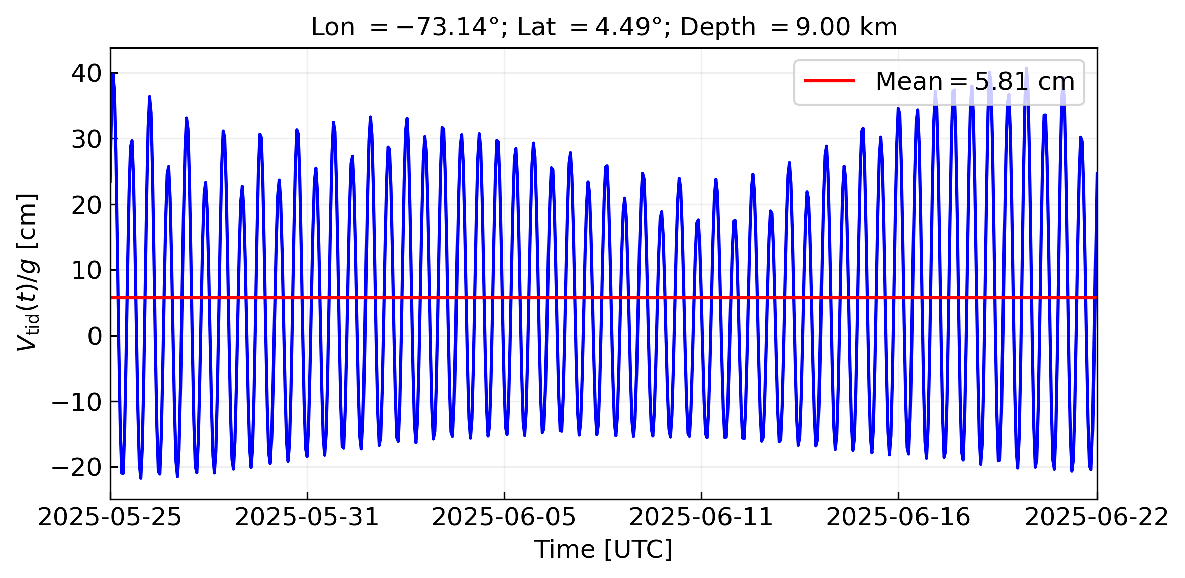
# Calculate TGP for a single body (Moon)
tgp_one, et_utc = earth.tgp_one_body('Moon', loc_sta=loc, dates=date, nmax=6, time_array=True)
Finally, plot the resulting signal:
# Plot the signal
earth.plot_one_signal(et_utc, tgp_one*100, loc=loc, colors=['blue','red'], mean_value=True,
                      savepath='./tgp-earth-moon.png')
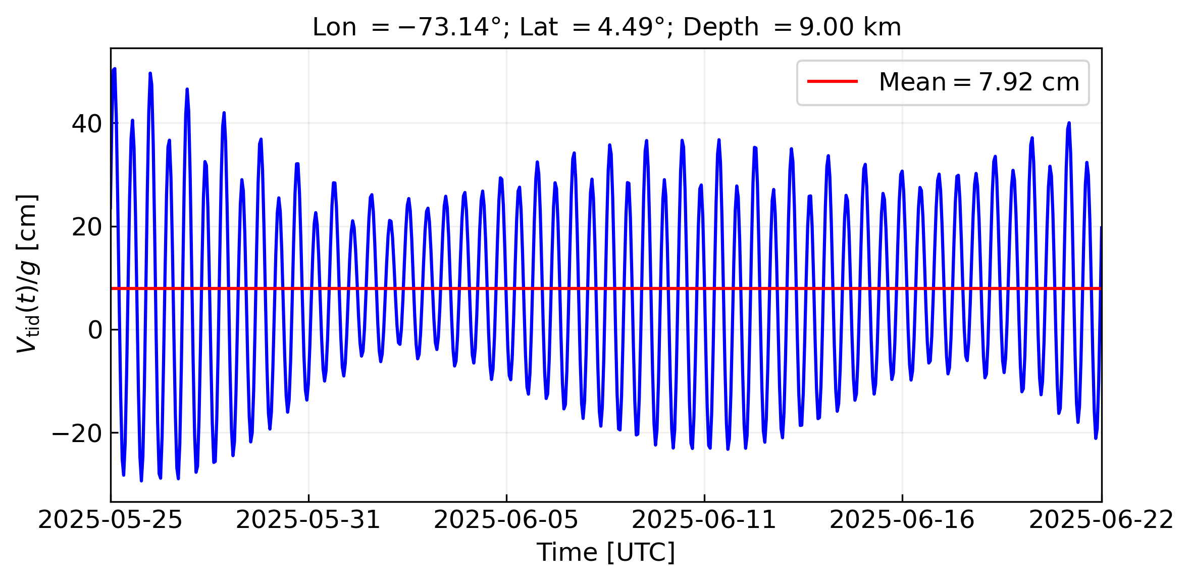
Multiple Bodies
You can also calculate the combined tidal potential from multiple celestial bodies:
# List of bodies
bodylist = ['Moon', 'Sun', 'Mercury', 'Venus', 'Mars Barycenter', 'Jupiter Barycenter']

# Calculate combined TGP
tgp_many = earth.tgp_many_bodies(bodylist, loc_sta=loc, dates=date, nmax=6, body_signal=False, time_array=False)

# Plot the combined signal
earth.plot_one_signal(et_utc, tgp_many*100, loc=loc, colors=['blue','red'], mean_value=True,
                      savepath='./tgp-earth-planets.png')
Calculating Planetary Response (Love Numbers)
tSPICE can also calculate the elastic response of a planetary body (Love numbers) by integrating interior models. Here is how to calculate the Love numbers $k_2, h_2, l_2$ for Earth using a modified PREM model:
First, initialize the package and define the responding body with its characteristic scales:
import tspice as tsp
from tspice.planet import Earth

# Initialize
tsp.initialize(verbose=False)

# Define responding body and characteristic scales
earth_interior = tsp.BodyResponse('Earth')
earth_interior.scale_constants()
Next, load a planetary profile. In this case, we use the Modified PREM for Earth:
earth_model = Earth()
planet_profile = earth_model.planet_profile
Define the internal layers of the planet (boundaries between fluid and solid regions matter):
# The fluid outer core is sandwiched between the solid inner core and mantle
layers_list = [
    dict(name='Outer Core', type='fluid', r0=1221500.0, rf=3480000.0),
    dict(name='Inner Core', type='solid', r0=0, rf=1221500.0),
    dict(name='Mantle + crust', type='solid', r0=3480000.0, rf=earth_interior.L)
]
Set the integration parameters for the desired tidal frequency (e.g., M2 tide) and spherical harmonic degree (n=2):
f_day = 1.93502  # cycles/day
earth_interior.set_integration_parameters_ad(n=2, f_days=f_day,
                                             layers_list=layers_list,
                                             planet_profile=planet_profile,
                                             r0_ini=6e3)
Finally, integrate the coupled ODEs and print the results:
# Integrate
earth_interior.integrate_internal_solutions_ad(verbose=True)

# Access computed Love numbers
print(f"k_2 = {earth_interior.k_n}, h_2 = {earth_interior.h_n}, l_2 = {earth_interior.l_n}")
# Output: k_2 = 0.2990433851603629, h_2 = 0.6093161139942496, l_2 = 0.08564339441970326
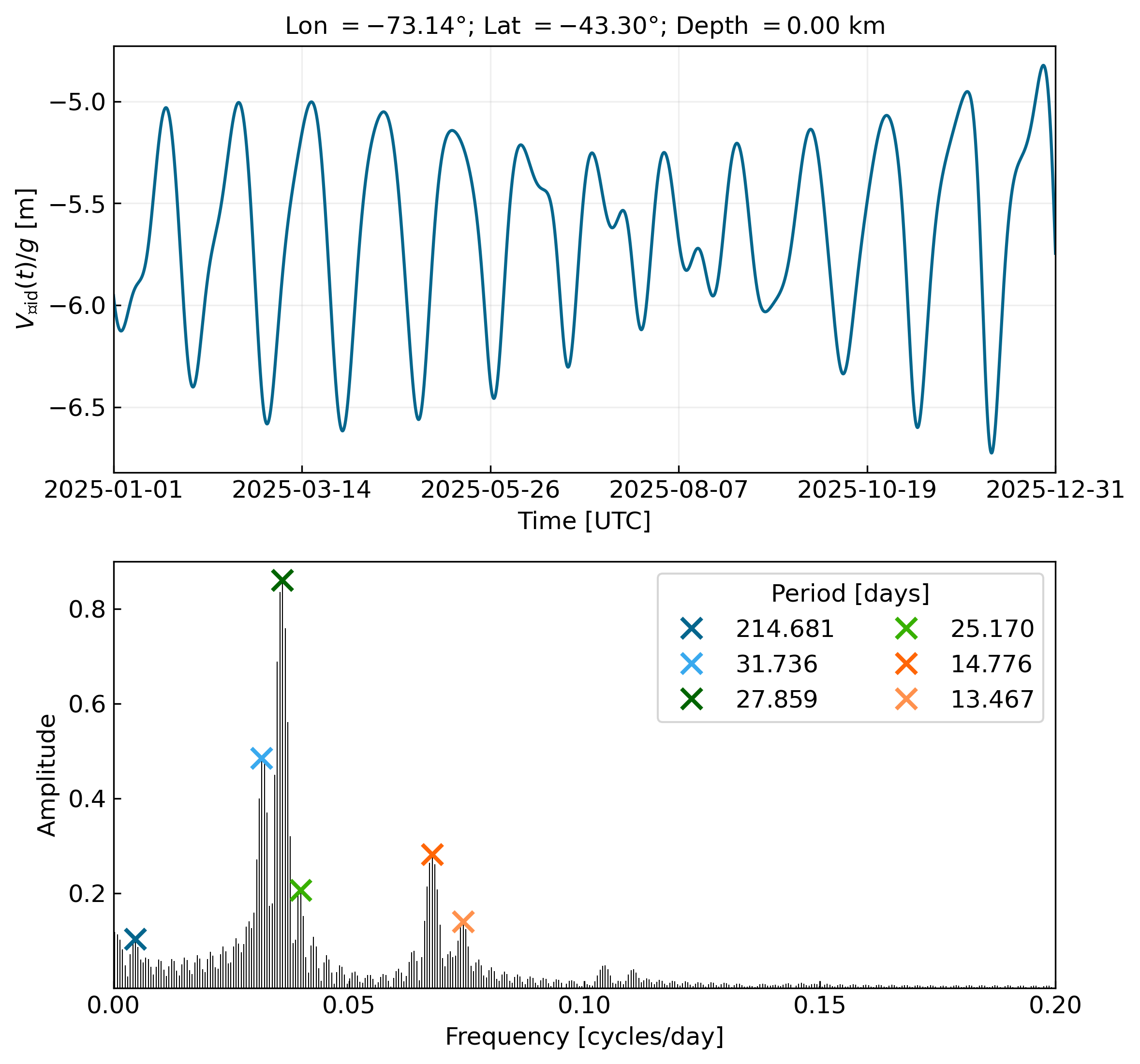
Spectral Analysis (Lomb-Scargle)
You can also analyze the spectral content of the tidal signal to identify the main tidal modes (e.g., monthly, fortnightly). Here is how to compute the Lomb-Scargle periodogram for the Moon's potential:
from astropy.timeseries import LombScargle
import astropy.units as u
from scipy.signal import find_peaks
import pandas as pd

# Prepare time array in days
t = (et_utc - et_utc.min()) / (3600 * 24)

# Compute Periodogram (assuming tgp_one is the Moon's potential)
frequency, power = LombScargle(t * u.day, tgp_one * u.m).autopower(maximum_frequency=0.2 * u.day**-1)
amplitude = (power.value)**0.5

# Find peaks
peaks_ind, _ = find_peaks(amplitude, height=0.06, prominence=0.076)
peaks_freq = frequency.value[peaks_ind]
peaks_amp = amplitude[peaks_ind]
peaks_period = 1 / peaks_freq

# Show main modes
df = pd.DataFrame({'Frequency (1/d)': peaks_freq,
                   'Period (d)': peaks_period,
                   'Amplitude': peaks_amp})
print(df.sort_values('Amplitude', ascending=False))
Visualizing the spectrum reveals the dominant periods (e.g., ~27 days for the Moon):
Authors
- Deivy Mercado - david231097@gmail.com
- Jorge I. Zuluaga - jorge.zuluaga@udea.edu.co
- Gloria Moncayo - gloria.moncayo@udea.edu.co
License
This project is licensed under the GNU Affero General Public License v3.0 (AGPL-3.0) - see the LICENSE file for details.
Release history Release notifications | RSS feed


Download files
Download the file for your platform. If you're not sure which to choose, learn more about installing packages.
Source Distribution
Built Distribution
Filter files by name, interpreter, ABI, and platform.
If you're not sure about the file name format, learn more about wheel file names.
Copy a direct link to the current filters
File details
Details for the file tspice-1.0.0.tar.gz.
File metadata
- Download URL: tspice-1.0.0.tar.gz
- Upload date:
- Size: 57.2 kB
- Tags: Source
- Uploaded using Trusted Publishing? No
- Uploaded via: twine/5.0.0 CPython/3.12.7
File hashes
| Algorithm | Hash digest | |
|---|---|---|
| SHA256 |
0ba327e3af7a6710de188760e7297df545eb3a649b526e1cf5799e8ed99b1e9d
|
|
| MD5 |
27d19b627d8f218cc2bc8c9c93f8b48c
|
|
| BLAKE2b-256 |
a5b912b286ee43ebe0501048ea83391210160d3b149b13db20f5e83717976451
|
File details
Details for the file tspice-1.0.0-py3-none-any.whl.
File metadata
- Download URL: tspice-1.0.0-py3-none-any.whl
- Upload date:
- Size: 51.9 kB
- Tags: Python 3
- Uploaded using Trusted Publishing? No
- Uploaded via: twine/5.0.0 CPython/3.12.7
File hashes
| Algorithm | Hash digest | |
|---|---|---|
| SHA256 |
f97c35340c1a794c686fb9d3933c90d7453430262f285db1b1d2bceeb7072a5d
|
|
| MD5 |
b3db97cf20e5dc5e0aaf3668f4415e0d
|
|
| BLAKE2b-256 |
b74e42f24dda7dadfdd1bb54437215b5fe3e202d2a981d7f1809183a02b26993
|


