uamc-spectrophore 1.2.0

Python implementation of the spectrophore descriptor

Spectrophores

This module contains python code to calculate spectrophores from molecules. It is using the RDKit and numba toolkits.

The technology and its applications have been described in Journal of Cheminformatics (2018) 10, 9. The paper is also included in this distribution.

The spectrophore code can be used in two ways:

• As a standalone program to convert the molecules in a sd-file into their corresponding spectrophores;
• As a python module to import in your own python code.

In the following sections, both usages will be documented.

Installation

1. Installation of RDKit and Numba

We recommend to install both RDKit and Numba using Anaconda. If conda is not yet available on your system, you should install this first following the instructions on the Anaconda website. Numba is an open source JIT compiler that translates a subset of Python and NumPy code into fast machine code. RDKit is open source cheminformatics software that provides the code to work with molecules.

The easiest way to have everything installed is using conda. First create a suitable environment in which you will install the spectrophore technology:

> conda create --name spectrophore python=3

This will install a new conda environment with Python 3.9 installed in it. Now activate this environment:

> conda activate spectrophore

Numba and rdkit can now be installed as follows (make sure you first activated the spectrophore environment):

> conda install numba
> conda install cudatoolkit
> conda install -c conda-forge rdkit

You can test the rdkit installation by opening a python session from your command-line (assuming you are still in the activated spectrophore environment) and typing the following:

>>> from rdkit import Chem
>>> mol = Chem.MolFromSmiles("C1CCCC1")
>>> print(mol.GetNumAtoms())
5

Similarly, you can test the numba installation with this small python snippet:

>>> import numba
>>> numba.__version__
'0.51.2'

With numba -s command you can also check whether you have a CUDA device installed (check for the section __CUDA Information__).

2. Installing the spectrophore code

With the spectrophore environment still active, you can now easily install the spectrophore module using:

> pip install uamc-spectrophore

Check the installation by opening a python session and entering:

>>> from spectrophore import spectrophore
>>> spectrophore.__version__
'1.2.0'

1. Usage as a standalone program

After installation, one should be able to use the spectrophore.py code as a standalone program to calculated spectrophores from a sd-file with molecules. You can find out where spectrophore.py is located by starting a python shell and typing:

>>> from spectrophore import spectrophore
>>> spectrophore.__file__
'/Users/hans/anaconda3/envs/spectrophore/lib/python3.8/site-packages/spectrophore/spectrophore.py'

Either you can use this full path to call the spectrophore.py code, or you can add it to your $PATH environment variable.

To use spectrophore.py, type the following on the command-line:

> spectrophore.py -h

This will provide you with all details on how to calculate spectrophores from a sd-file:

usage: spectrophore.py [-h] [-n {none,mean,all,std}] [-s {none,unique,mirror,all}] [-a {1,2,3,4,5,6,9,10,12,15,18,20,30,36,45,60,90,180}]
                       [-r RESOLUTION] [-p MAX_WORKERS] -i INFILE -o OUTFILE

Calculate spectrophores

optional arguments:
  -h, --help            show this help message and exit
  -n {none,mean,all,std}, --norm {none,mean,all,std}
                        normalization setting (default: all)
  -s {none,unique,mirror,all}, --stereo {none,unique,mirror,all}
                        stereo setting (default: none)
  -a {1,2,3,4,5,6,9,10,12,15,18,20,30,36,45,60,90,180}, --accuracy {1,2,3,4,5,6,9,10,12,15,18,20,30,36,45,60,90,180}
                        accuracy setting (default: 20)
  -r RESOLUTION, --resolution RESOLUTION
                        resolution setting (>0) (default: 3)
  -p MAX_WORKERS, --np MAX_WORKERS
                        number of processors to use; -1 is all processors (default: -1)

required arguments:
  -i INFILE, --in INFILE
                        input sdf file (default: None)
  -o OUTFILE, --out OUTFILE
                        output spectrophore file (default: None)

2. Usage as a python module

2.1. Introduction

Once you have installed all required tools and the uamc-spectrophore package, you are ready to use the tool. In its most simple form, spectrophores can be calculated as follows:

>>> from spectrophore import spectrophore
>>> from rdkit import Chem
>>> from rdkit.Chem import AllChem
>>> mol = Chem.MolFromSmiles("c1ncncc1")
>>> mol = Chem.AddHs(mol)
>>> AllChem.EmbedMolecule(mol, randomSeed=1)
0
>>> calculator = spectrophore.SpectrophoreCalculator(normalization='none')
Probes initialised: 48 number of probes in total
12 probes are used due to the imposed stereo flag
>>> calculator.calculate(mol)
array([  1.409246  ,   2.021652  ,   1.6011626 ,   3.034698  ,
         2.4150815 ,   5.0872273 ,   2.285813  ,   1.7250485 ,
         3.436644  ,   4.0012817 ,   5.092206  ,   2.9844987 ,
         0.6417792 ,   0.8024898 ,   4.8707156 ,   4.870761  ,
         2.8789856 ,   4.104702  ,   1.9413302 ,   3.5960448 ,
         4.9019723 ,   4.151822  ,   4.5394773 ,   5.766127  ,
        44.79124   ,  71.551796  , 106.82244   , 106.82059   ,
        49.73703   ,  61.662792  ,  23.50798   ,  81.88448   ,
        77.47026   ,  67.52185   ,  57.44229   , 112.96884   ,
         0.6794604 ,   1.1607243 ,   2.470075  ,   2.470103  ,
         1.0203087 ,   1.1483352 ,   0.51142335,   1.7433033 ,
         1.8094715 ,   1.3015395 ,   1.2431506 ,   2.5163455 ],
      dtype=float32)

In the example shown, the first three lines import the required modules: module spectrophore for the calculation of spectrophores, module Chem to generate a RDKit molecule from a smiles string, and module AllChem to generate a 3D-conformation from the molecule. Next, a molecule is created from a smiles string (line 4), and a conformation is then generated at the 6'th line after adding hydrogen atoms on the 5'th line. Finally, on lines 7 and 8, a SpectrophoreCalculator object is generated and this object is then used to calculate a spectrophore descriptor (line 8), which consists in its default form of 4 * 12 numbers.

Note: a few words on the shape of a spectrophore:

Each spectrophore consists of a set of floating point numbers, and this set is always a multiple of 4. The actual number count depends on how stereochemistry is treated in the calculation of spectrophores; this is controlled by the stereo() method:

• stereo("none"): the total number of numbers in a spectrophore is 48 (4 * 12; default),
• stereo("unique"): the total number of numbers in a spectrophore is 72 (4 * 18),
• stereo("mirror"): the total number of numbers in a spectrophore is 72 (4 * 18),
• stereo("all"): the total number of numbers in a spectrophore is 144 (4 * 36).

Whatever the actual number of spectrophore points, these are always calculated according the same atomic properties. For example, consider a spectrophore of 4n points, then these points represent the following:

• Points 1 to n: representing the interaction energies between the atomic partial charges and each of the n boxes;
• Points n+1 to 2n: representing the interaction energies between the atomic lipophilicities and each of the n boxes;
• Points 2n+1 to 3n: representing the interaction energies between the atomic shape deviations and each of the n boxes;
• Points 3n+1 to 4n: representing the interaction energies between the atomic electrophilicities and each of the n boxes.

Please have a look at the original publication form more information about the way these interaction energies are calculated, and what the stereo() method actually means.

If a molecule contains more than one 3D-conformation, then one may specify which conformation should be used for the calculation of spectrophores. As an example, consider the following code:

>>> calculator = spectrophore.SpectrophoreCalculator(normalization='none')
Probes initialised: 48 number of probes in total
12 probes are used due to the imposed stereo flag
>>> aspirin = Chem.MolFromSmiles("CC(Oc1ccccc1C(O)=O)=O")
>>> mol = Chem.AddHs(mol)
>>> cids = AllChem.EmbedMultipleConfs(aspirin, numConfs=3, randomSeed=1)
>>> print(len(cids))
3
>>> for i in range(len(cids)): calculator.calculate(aspirin, i)
...
array([  2.964628 ,   3.1078947,   2.927014 ,   4.7348037,   7.507005 ,
         6.7752705,   4.694607 ,   4.9843326,   6.566493 ,   8.246073 ,
        10.165346 ,   6.63523  ,   4.858508 ,   8.002102 ,   6.8100824,
         8.816333 ,  15.715073 ,  19.571812 ,  10.928973 ,  14.395827 ,
        17.003227 ,  18.447824 ,  25.714355 ,  15.146796 ,  72.9549   ,
        98.34449  , 169.34996  , 182.39804  , 131.36954  , 131.15866  ,
        65.37012  , 130.0362   , 162.26236  , 149.89626  , 179.36638  ,
       198.5693   ,   2.2463505,   3.1564593,   5.1663566,   5.612588 ,
         4.058919 ,   4.409714 ,   2.2037854,   4.4034805,   4.9583206,
         5.239315 ,   5.461795 ,   6.264689 ], dtype=float32)
array([  2.863708 ,   3.1190798,   2.9663007,   4.770968 ,   7.393107 ,
         7.3158054,   4.9012723,   5.10262  ,   6.548969 ,   8.572092 ,
        10.425214 ,   6.4823613,   4.787042 ,   8.08808  ,   6.631177 ,
         8.741646 ,  16.067795 ,  19.49238  ,  10.819519 ,  14.260894 ,
        16.789541 ,  18.33067  ,  25.610632 ,  14.279321 ,  69.21315  ,
        96.67396  , 170.67822  , 184.54782  , 119.22876  , 135.03757  ,
        59.888947 , 119.49558  , 173.35124  , 145.16624  , 180.47777  ,
       187.60854  ,   2.1962543,   3.108443 ,   5.2100787,   5.6747303,
         3.8506951,   4.435027 ,   2.1061015,   4.0988173,   5.171605 ,
         5.103154 ,   5.384299 ,   5.955127 ], dtype=float32)
array([  3.0309825,   3.435472 ,   2.8768196,   4.706544 ,   7.5557814,
         6.4479575,   4.55689  ,   4.953575 ,   6.4871607,   8.706506 ,
         8.518427 ,   6.3662963,   4.9284625,   9.355401 ,   6.6179686,
         8.523829 ,  15.459739 ,  19.284777 ,  10.792515 ,  13.991817 ,
        16.795666 ,  18.597605 ,  24.084375 ,  13.117221 ,  77.639145 ,
       120.10927  , 169.49625  , 166.18648  , 131.14139  , 144.46242  ,
        72.4695   , 149.30933  , 140.35475  , 155.59204  , 130.84991  ,
       174.86932  ,   2.4413445,   3.8801153,   5.1489463,   4.834638 ,
         4.0795846,   4.013626 ,   2.4914305,   4.5840054,   4.270138 ,
         5.335861 ,   4.6315002,   5.6371183], dtype=float32)

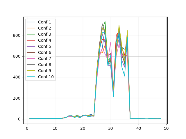
One can easily visualise spectrophores by plotting the actual values. For example, consider the following snippet:

>>> import matplotlib.pyplot as plt
>>> mol = Chem.MolFromSmiles("CC(CCC1=CC=CC=C1Cl)N1CCOCC1")
>>> mol = Chem.AddHs(mol)
>>> cids = AllChem.EmbedMultipleConfs(mol, numConfs = 10, randomSeed = 1)
>>> spectrophores = []
>>> for cid in cids: spectrophores.append(calculator.calculate(mol, cid))
...
>>> for i in range(len(spectrophores)): plt.plot(range(1,49), spectrophores[i], label='Conf %d' % (i+1))
...
[<matplotlib.lines.Line2D object at 0x7f989dc3f4f0>]
[<matplotlib.lines.Line2D object at 0x7f989dc3f850>]
[<matplotlib.lines.Line2D object at 0x7f989dc3fbb0>]
[<matplotlib.lines.Line2D object at 0x7f989dc3ff10>]
[<matplotlib.lines.Line2D object at 0x7f989dc512b0>]
[<matplotlib.lines.Line2D object at 0x7f989dc51610>]
[<matplotlib.lines.Line2D object at 0x7f989dc51970>]
[<matplotlib.lines.Line2D object at 0x7f989dc51cd0>]
[<matplotlib.lines.Line2D object at 0x7f989dc5e070>]
[<matplotlib.lines.Line2D object at 0x7f989dc5e3d0>]
>>> plt.legend(loc='upper left')
<matplotlib.legend.Legend object at 0x7f9899470e80>
>>> plt.grid()
>>> plt.savefig("spectrophore/images/exampleplot1.png")

which generates the following plot:

Similarly, one can easily compare the spectrophores from two different molecules, and quantify the difference:

>>> plt.close()
>>> spectrophores = []
>>> mols = [Chem.MolFromSmiles("ClC(Br)(I)F"), Chem.MolFromSmiles("CC(CCC1=CC=CC=C1Cl)N1CCOCC1")]
>>> for i in range(2):
...    mols[i] = Chem.AddHs(mols[i])
...    AllChem.EmbedMolecule(mols[i], randomSeed=1)
...    spectrophores.append(calculator.calculate(mols[i]))
...
0
0
>>> for i in range(2): plt.plot(range(1,49), spectrophores[i], label='Molecule %d' % (i+1))
...
[<matplotlib.lines.Line2D object at 0x7faf420df520>]
[<matplotlib.lines.Line2D object at 0x7faf420df4c0>]
>>> plt.grid()
>>> plt.savefig("spectrophore/images/exampleplot2.png")
>>> from scipy.spatial import distance
>>> distance.euclidean(spectrophores[0],spectrophores[1])
2060.65478515625

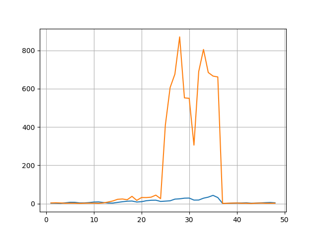
From the last example, it is clear that the actual spectrophore values may differ a lot depending on the type of molecule. Also, the absolute values are depending on the property type, with some properties leading to large values (e.g. shape deviation) and others very small. For this reason, a number of normalisation methods are provided as shown below.

2.2. Module methods

resolution()

The resolution() method controls the smallest distance between the molecule and the surrounding box. By default this value is set to 3.0 A. The resolution() can be specified at the moment of class creation, or later on using the resolution() method:

>>> mol = Chem.MolFromSmiles("ClC(Br)(I)F")
>>> AllChem.EmbedMolecule(mol, randomSeed=1)
0
>>> calculator = spectrophore.SpectrophoreCalculator(normalization='none')  # Default of 3.0
Probes initialised: 48 number of probes in total
12 probes are used due to the imposed stereo flag
>>> print(calculator.calculate(mol)[0])
2.9869986
>>> calculator = spectrophore.SpectrophoreCalculator(normalization='none', resolution = 3.0)
Probes initialised: 48 number of probes in total
12 probes are used due to the imposed stereo flag
>>> print(calculator.calculate(mol)[0])
2.9869986
>>> calculator = spectrophore.SpectrophoreCalculator(normalization='none', resolution = 5.0)
Probes initialised: 48 number of probes in total
12 probes are used due to the imposed stereo flag
>>> print(calculator.calculate(mol)[0])
1.341883
>>> calculator.resolution(10.0)
>>> print(calculator.calculate(mol)[0])
0.3347178

The larger the resolution value (e.g. 10.0 versus 3.0 A), the smaller the interaction energies and corresponding spectrophore values.

Calling the resolution() method without an argument returns the current resolution value:

>>> calculator.resolution()
10.0

accuracy()

The accuracy() method controls the angular stepsize by which the molecule is rotated within the cages. By default this value is set to 20°. This parameter can be modified either at class creation, or using the accuracy() method later on. The accuracy should be an integer fraction of 180, hence 180 modulus accuracy should be equal to 0. The smaller the accuracy value (meaning smaller angular stepsizes), the longer the computation time:

>>> calculator = spectrophore.SpectrophoreCalculator(accuracy = 20.0, normalization = 'none') # Default
Probes initialised: 48 number of probes in total
12 probes are used due to the imposed stereo flag
>>> print(calculator.calculate(mol)[0])
2.9869986
>>> calculator = spectrophore.SpectrophoreCalculator(normalization = 'none')
Probes initialised: 48 number of probes in total
12 probes are used due to the imposed stereo flag
>>> print(calculator.calculate(mol)[0])
2.9869986
>>> calculator = spectrophore.SpectrophoreCalculator(accuracy = 2.0, normalization = 'none')
Probes initialised: 48 number of probes in total
Only using 12 probes
>>> print(calculator.calculate(mol)[0])    # Takes some time
3.0315504
>>> 100.0 * (3.0315504 - 2.9869986) / 3.0315504
1.469604463775361

Calling the accuracy() method without an argument returns the current accuracy value:

>>> calculator.accuracy()
2

normalization()

With the normalization() method, one can specify the type of spectrophore normalization. There are four possibilities:

• normalization("none"): no normalization is applied and the spectrophore values are the raw calculated interaction energies (multiplied by -100),
• normalization("mean"): for each property, the average value is calculated and each of the individual spectrophore property value are reduced by these mean values. This centers the calculated values around 0,
• normalization("std"): for each property, the standard deviation is calculated and each of the individual spectrophore property value is divided by these standard deviations,
• normalization("all"): each spectrophore value is normalized by mean and standard deviation. This is the fefault option.

The default value is "all".

>>> calculator.accuracy(20)
>>> calculator.normalization("none")
>>> spec = calculator.calculate(mol)
>>> print(spec[:12])
[2.9869986 2.7023215 1.8029709 4.468909  7.3755445 7.2522745 4.1123347
 4.0559936 5.9084597 8.5649605 9.328256  6.22969  ]
>>> sum(spec[:12])
64.78871297836304
>>> calculator.normalization("mean")
>>> spec = calculator.calculate(mol)
>>> print(spec[:12])
[-2.4120607  -2.6967378  -3.5960884  -0.9301505   1.9764853   1.8532152
 -1.2867246  -1.3430657   0.50940037  3.1659012   3.9291964   0.8306308 ]
>>> sum(spec[:12])
1.430511474609375e-06
>>> calculator.normalization("std")
>>> spec = calculator.calculate(mol)
>>> print(spec[:12])
[1.2924111 1.1692374 0.7801074 1.9336023 3.1912422 3.1379058 1.7793202
 1.7549427 2.5564656 3.7058773 4.036139  2.695455 ]
>>> sum(spec[:12])
28.032706141471863
>>> calculator.normalization("all")
>>> spec = calculator.calculate(mol)
>>> print(spec[:12])
[-1.0436476  -1.1668214  -1.5559514  -0.40245646  0.85518336  0.80184704
 -0.5567385  -0.58111614  0.22040677  1.3698184   1.7000802   0.35939637]
>>> sum(spec[:12])
6.854534149169922e-07

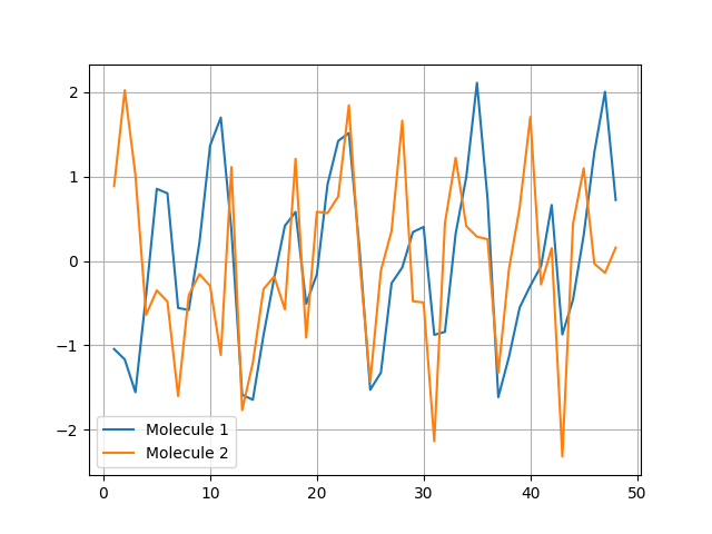
Using a normalization over 'all' makes it more easier to compare spectrophores between molecules:

>>> plt.close()
>>> mols = [Chem.MolFromSmiles("ClC(Br)(I)F"), Chem.MolFromSmiles("CC(CCC1=CC=CC=C1Cl)N1CCOCC1")]
>>> spectrophores = []
>>> for i in range(2):
...    mols[i] = Chem.AddHs(mols[i])
...    AllChem.EmbedMolecule(mols[i], randomSeed = 1)
...    spectrophores.append(calculator.calculate(mols[i]))
...
0
0
>>> for i in range(2): plt.plot(range(1,49), spectrophores[i], label='Molecule %d' % (i+1))
...
[<matplotlib.lines.Line2D object at 0x7faf420df520>]
[<matplotlib.lines.Line2D object at 0x7faf420df4c0>]
>>> plt.legend()
<matplotlib.legend.Legend object at 0x7f989ed85820>
>>> plt.grid()
>>> plt.savefig("spectrophore/images/exampleplot3.png")
>>> from scipy.spatial import distance
>>> distance.euclidean(spectrophores[0],spectrophores[1])
8.374645233154297

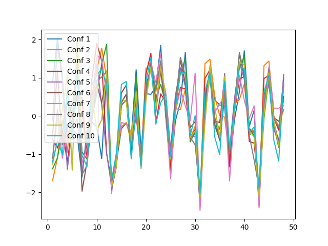
The same holds true when comparing spectrophores from different conformations:

>>> plt.close()
>>> spectrophores = []
>>> mol = Chem.MolFromSmiles("CC(CCC1=CC=CC=C1Cl)N1CCOCC1")
>>> mol = Chem.AddHs(mol)
>>> cids = AllChem.EmbedMultipleConfs(mol, numConfs = 10, randomSeed = 1)
>>> calculator.normalization("all")
>>> for cid in cids: spectrophores.append(calculator.calculate(mol, cid))
...
>>> for i in range(len(spectrophores)): plt.plot(range(1,49), spectrophores[i], label='Conf %d' % (i+1))
...
[<matplotlib.lines.Line2D object at 0x7f989f9cc070>]
[<matplotlib.lines.Line2D object at 0x7f989f9cc3d0>]
[<matplotlib.lines.Line2D object at 0x7f989f9cc730>]
[<matplotlib.lines.Line2D object at 0x7f989f9cca90>]
[<matplotlib.lines.Line2D object at 0x7f989f9ccdf0>]
[<matplotlib.lines.Line2D object at 0x7f989f9d8190>]
[<matplotlib.lines.Line2D object at 0x7f989f9d84f0>]
[<matplotlib.lines.Line2D object at 0x7f989f9d8850>]
[<matplotlib.lines.Line2D object at 0x7f989f9d8bb0>]
[<matplotlib.lines.Line2D object at 0x7f989f9d8f10>]
>>> plt.legend(loc='upper left')
<matplotlib.legend.Legend object at 0x7f989f948e50>
>>> plt.savefig("spectrophore/images/exampleplot4.png")
>>> from scipy.spatial import distance
>>> distance.euclidean(spectrophores[0],spectrophores[1])
5.974719524383545
>>> distance.euclidean(spectrophores[0],spectrophores[2])
6.081935882568359
>>> distance.euclidean(spectrophores[1],spectrophores[2])
3.7508902549743652

stereo()

The stereo() method specifies the kind of cages to be used. The reason for this is that some of the cages that are used to calculate spectrophores have a stereospecific distribution of the interaction points:

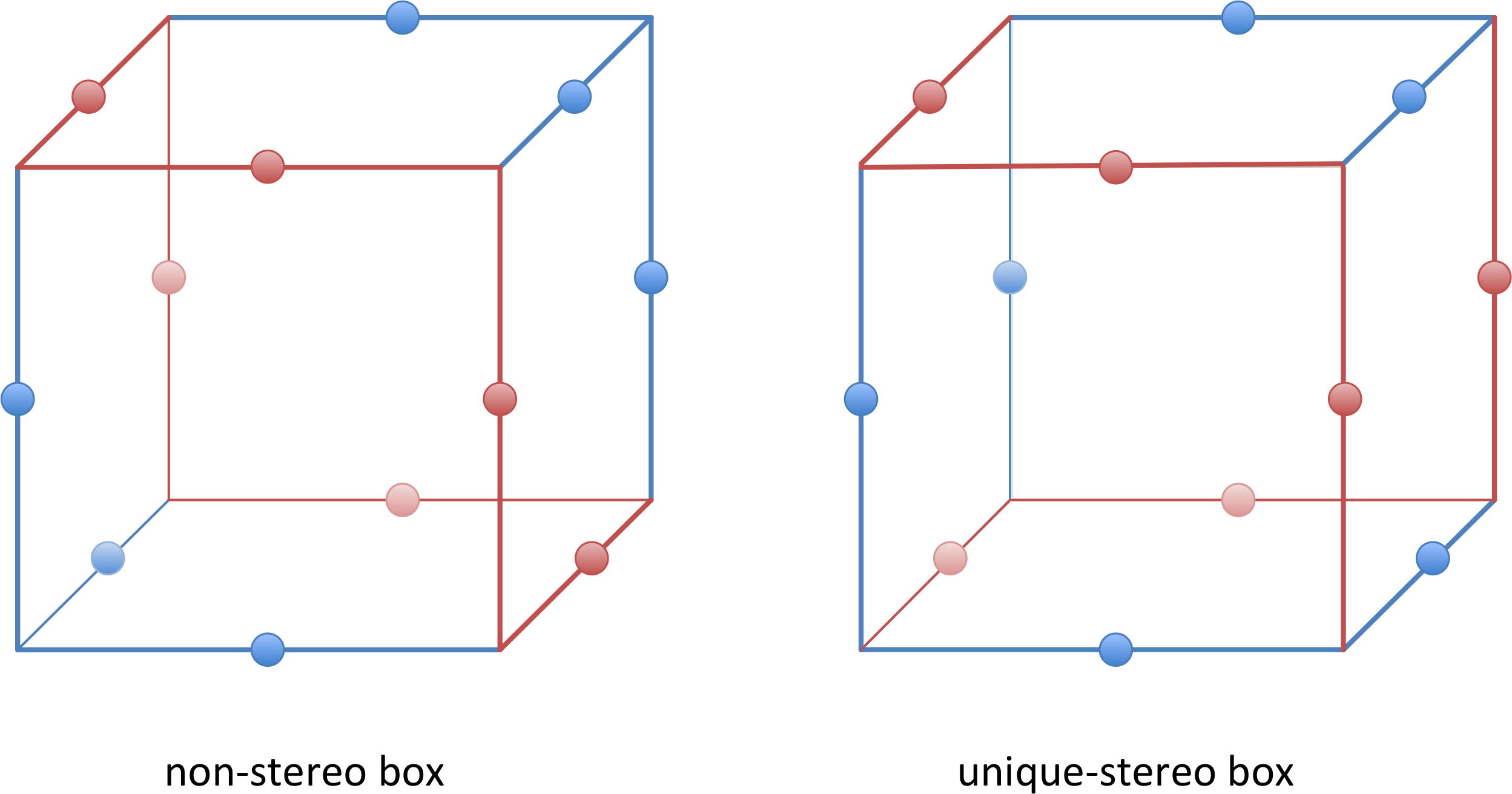
There are four possibilities:

• stereo("none"): no stereospecificity (default). Spectrophores are generated using cages that are not stereospecific. For most applications, these spectrophores will suffice,
• stereo("unique"): unique stereospecificity. Spectrophores are generated using unique stereospecific cages,
• stereo("mirror"): mirror stereospecificity. Mirror stereospecific spectrophores are spectrophores resulting from the mirror enantiomeric form of the input molecules,
• stereo("all"): all cages are used. This results in the longest spectrophores and should only in specific cases be used.

The differences between the corresponding data points of unique and mirror stereospecific spectrophores are very small and require very long calculation times to obtain a sufficiently high quality level. This increased quality level is triggered by the accuracy setting and will result in calculation times being increased by at least a factor 100. As a consequence, it is recommended to apply this increased accuracy only in combination with a limited number of molecules, and when the small differences between the stereospecific spectrophores are really critical. However, for the vast majority of virtual screening applications, this increased accuracy is not required as long as it is not the intention to draw conclusions about differences in the underlying molecular stereoselectivity. Non-stereospecific spectrophores will therefore suffice for most applications.

3. Interpreting spectrophores

A spectrophore is a vector of real number and has a certain length. The length depends on the used stereo method and the number of properties. The standard setting uses a set of non-stereospecific probes in combination with four properties:

• property 1: atomic partial charges
• property 2: atomic lipophilicities
• property 3: atomic shape deviations
• property 4: atomic electrophilicties

The combination of four properties and the set of non-stereospecific probes leads to a spectrophore vector length of 48. The use of other probes leads to other vector lengths, as summarised in this table:

Stereospecificity	Number of probes	Number of properties	Length
none	12	4	48
unique	18	4	72
mirror	18	4	72
all	36	4	144

The general layout of a spectrophore, irrespective of its length, is always:

Property 1	Property 2	Property 3	Property 4
probe 1..probe n	probe 1..probe n	probe 1..probe n	probe 1..probe n

meaning that the first n values (with n being the number of probes) are calculated using property 1 (partial charges), then another n values (n+1 up to 2n) calculated using property 2 (lipophilicities), and so forth.

4. Release updates

• 1.2.0:

  • Switched to numpy.float32 type to achieve major speedup

• 1.1.0:

  • Updated and optimised the NumPy code
  • Bug fixes
  • Introduced Numba
  • Made the 'all' normalization method the default one
  • Added a test suite

• 1.0.1: First official release on PyPi

5. Reference and citation

If you use the spectrophore technology in your own research work, please cite as follows:

Gladysz, R.; Mendes Dos Santos, F.; Langenaeker, W.; Thijs, G.; Augustyns, K.; De Winter, H. (2018) 'Spectrophores as one-dimensional descriptors calculated from three-dimensional atomic properties: applications ranging from scaffold hopping to multi-target virtual screening', J. Cheminformatics 10, 9.