
Library for handling Ulianov elliptical functions

Project description
UlianovEllipse
Example of Poliana Elliptical Flower, Duda Elliptical Flowers, and Salete Elliptical Flowers drawing using functions ulianov_ellipse_ue and ellipse_ab available in the UlianovEllipse library:
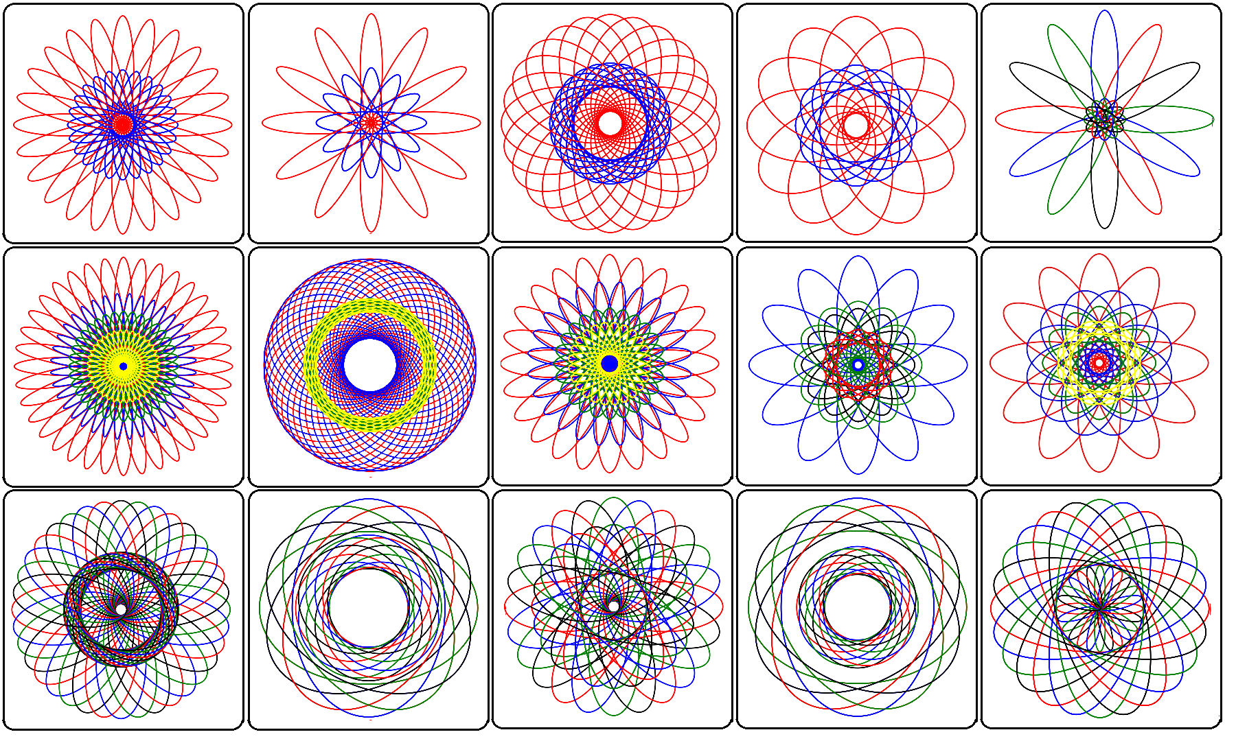
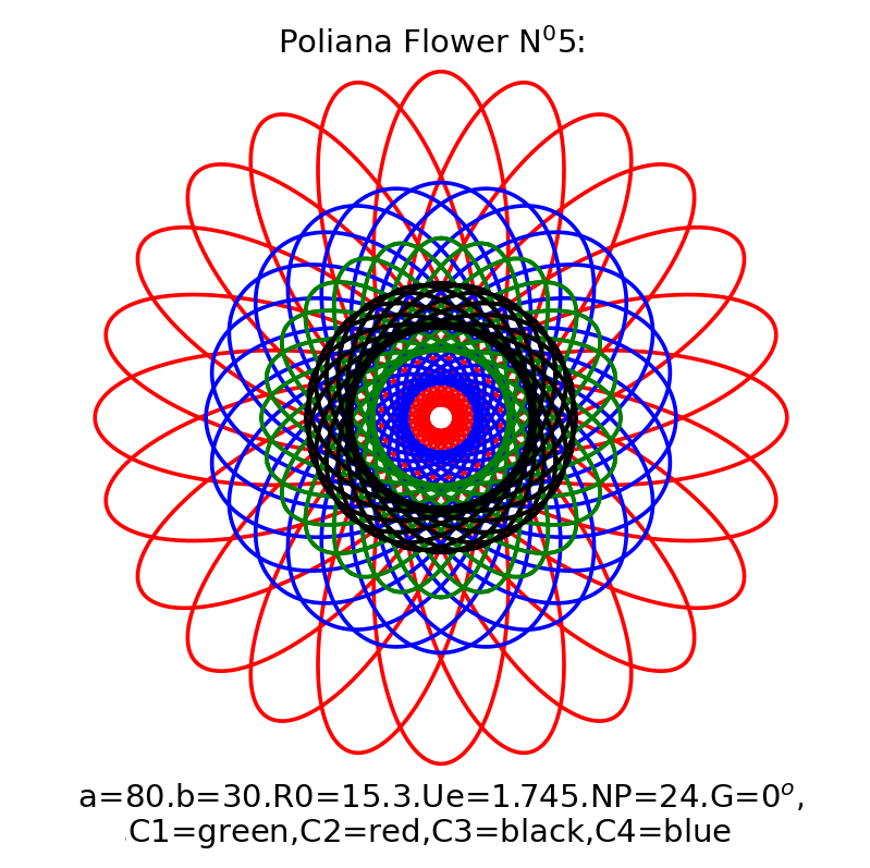
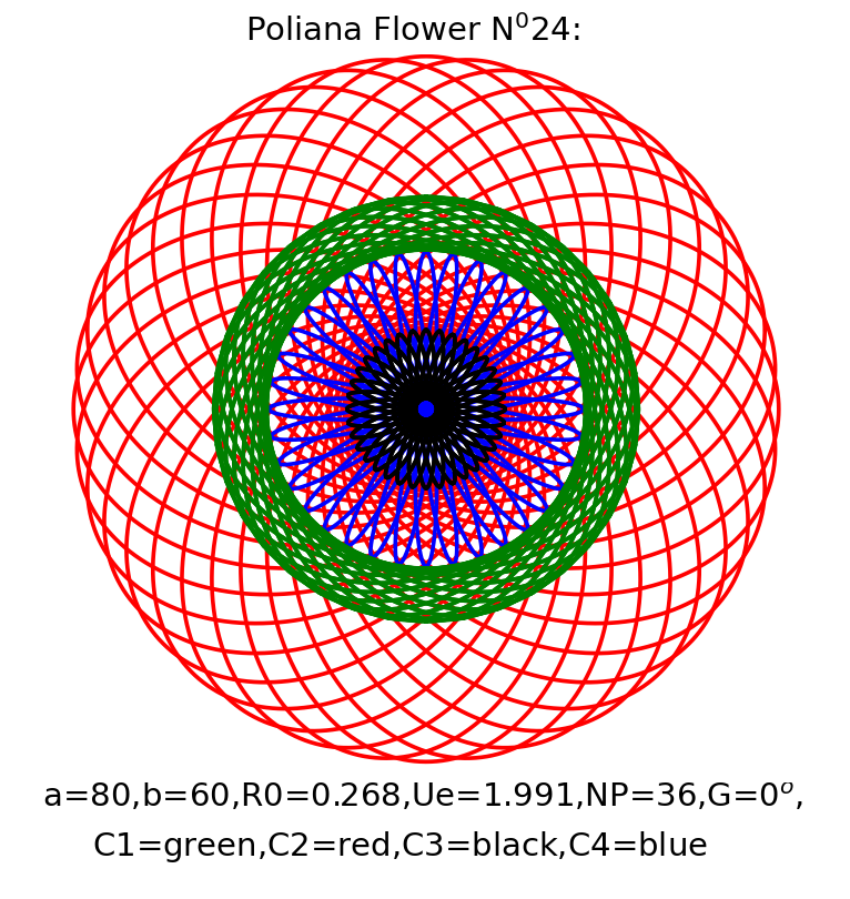
Poliana Elliptical Flover: Digital flower created by a python code that has a elliptical complex flower pattern, using two layers of ellipses (standard ellipse and Ulianov ellipse) with different size and color parameters, drawing using functions ulianov_ellipse_ue and ellipse_ab available in the UlianovEllipse library:
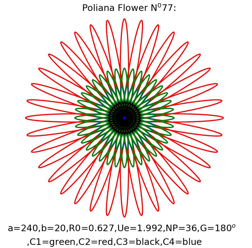
Poliana Elliptical Flover Zoom:
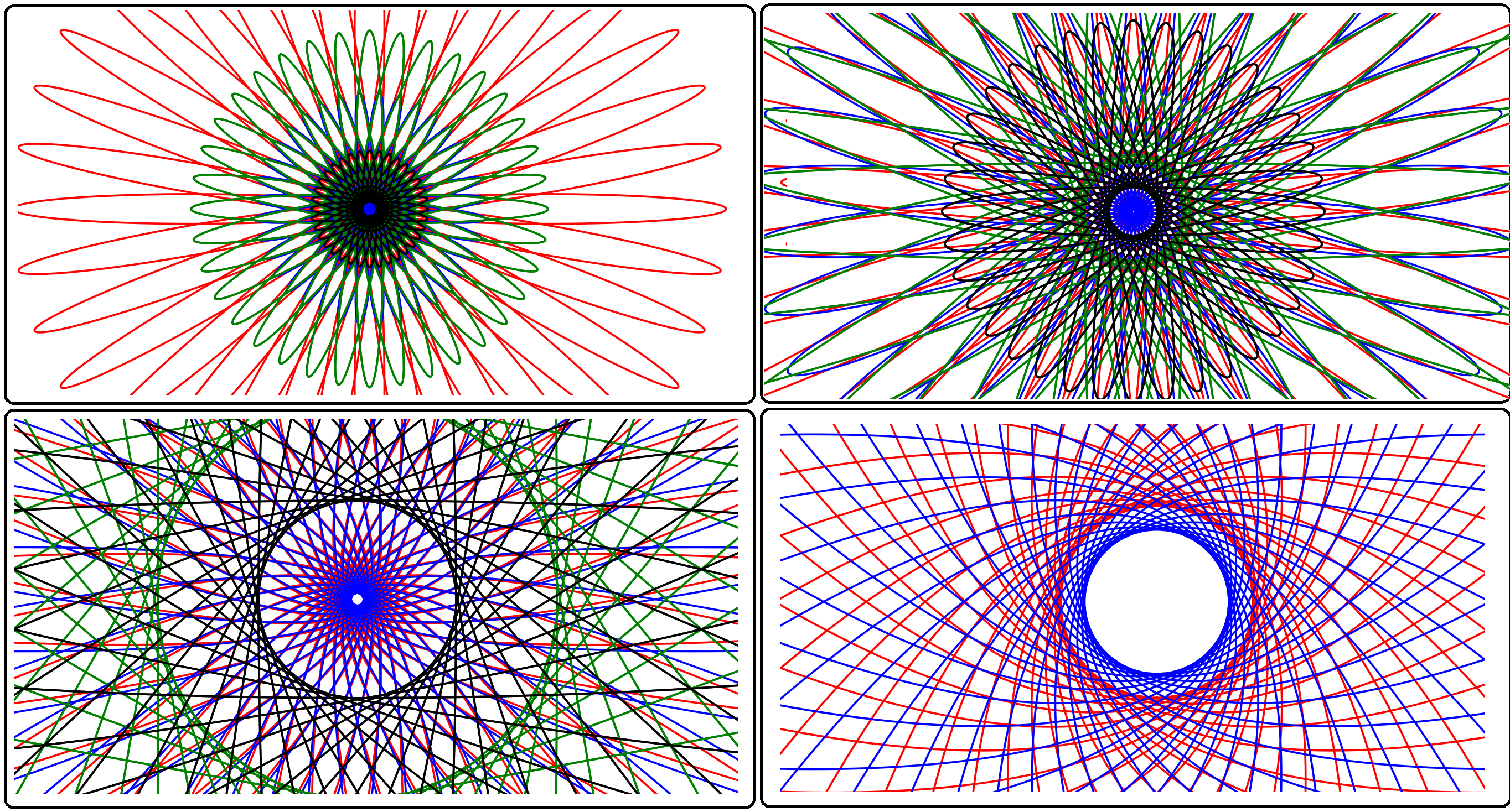
Overview
The UlianovEllipse library provides a comprehensive set of functions and classes for working with Ulianov elliptical functions. These functions are utilized in the Ulianov Orbital Model (UOM) to analyze and model elliptical orbits. The library also includes general utilities for handling and transforming elliptical shapes in various applications.
Key Features
- Ulianov Elliptical Cosine and Sine Functions: These functions (cosuell, sinuell) are used to calculate the cosine and sine of an angle for Ulianov ellipses, which differ from standard trigonometric functions.
- Parameter Conversion: Methods like calc_ue and calc_ab convert between different sets of parameters (semi-major "a" and semi-minor axes "b" parametres to Ulianov parameters "R0" and "Ue").
- Ulianov Elliptical Arctangent Functions: The arctanuell and arctanuell_ue functions allow the calculation of angles and parameters ("R0" and "Ue") from a given (x, y) point on the ellipse.
- Standard Ellipse Path Calculations: Functions such as ellipse_ue and ellipse_ab provide tools for calculating points along an ellipse using standard parameterizations ("a" and "b").
- Ulianov Ellipse Path Calculations: Functions such as ulianov_ellipse_ue and ulianov_ellipse_ab provide tools for calculating points along an ellipse using Ulianov Ellipse parameterizations ("R0" and "Ue").
Getting Started
To use the UlianovEllipse library, first ensure you have numpy installed, as it is a required dependency. You can install it using pip:
pip install numpy
pip install ulianovellipse
To see examples of use, go to the Examples of use section at the end of this document.
Technical Reference Manual for the ulianovellipse.py Library
Theoretical Basis
In the standard ellipse model, an ellipse is defined by two parameters, a and b:
(x/a)^2 + (y/b)^2 = 1
x = a cos(α)
y = b sin(α)
This equations define an ellipse over the (x,y) plane, centered at the origin (0,0), which intersects the x and y axes at the points: x = a, y = 0; x = 0, y = b; x = -a, y = 0; x = 0, y = -b. This ellipse is straightforward to implement, but in some cases (such as the orbits of planets around the sun), the ellipse must be centered at one of the foci, and the angle is defined differently.
In the Ulianov ellipse model, the same ellipse is defined using a parameter called the Ulianov Elliptic Parameter Ue:
R_0 = a - sqrt(a^2 - b^2)
Ue = b/(a R_0)
which allows for easily creating an ellipse:
x = R_0 cosuell(α, Ue)
y = R_0 sinuell(α, Ue)
This generates an ellipse identical to the one defined using a and b, but shifted to the left along the x-axis, with the center at x = R_0 - a, y = 0. It varies along the x-axis from x = -2a + R_0 to x = R_0 and along the y-axis from y = -b to y = b.
Knowing R_0 and Ue, the standard parameters are calculated by:
a = R_0/2 - Ue
b = R_0/sqrt((2/Ue) - 1)
Thus, using a, b or R_0, Ue is equivalent because one system can easily be converted to the other. However, it should be noted that the ellipse drawing will be shifted, and the angle α is defined differently when moving from the standard ellipse model to the Ulianov ellipse.
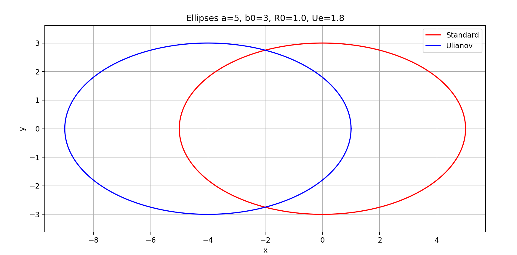
Observation: The Ulianov ellipse model generates ellipses only for 0 < Ue < 2. Ue = 0 generates a line on the x-axis, Ue = 1 generates a circle, Ue = 2 generates a parabola, and Ue > 2 generates hyperbolas. For ellipses (Ue between 0 and 2), the value of a must be greater than b to generate an ellipse with both foci on the x-axis. If b is greater than a, it results in a negative root in the calculation of R_0. To avoid this, a swap of the x and y axes is defined by swapping a with b. To signal this swap, the value of Ue is multiplied by -1. For example, the ellipse a = 5, b = 3 generates R_0 = 1, Ue = 1.8. In the case of b > a, the ellipse a = 3, b = 5 generates R_0 = 1, Ue = -1.8. In this case, the Ulianov ellipse is shifted downward with the center at x = 0, y = R_0 - b, varying from x = -a to x = a and from y = R_0 - 2b to R_0. Thus, for negative Ue, the ellipse is rotated 90 degrees.
This Ulianov ellipse model has an additional advantage: Given a point x, y on the ellipse and the parameter Ue, the value of α and R_0 can be determined:
α, R_0 = arctanuell(y, x, Ue)
Furthermore, if x, y, R_0 are known, it can be calculated:
α, Ue = arctanuell_ue(y, x, R_0)
For the standard ellipse, the angle α can be calculated using a scaling factor:
xi = x/a = cos(α)
yi = y/b = sin(α)
α = arctan2(yi, xi) = arctan2(y/b, x/a)
But in this case, both parameters a, b need to be known, and the angle α is defined concerning the geometric center of the ellipse. In the arctanuell and arctanuell_ue functions, only one parameter (R0 or Ue) needs to be known, and the angle defined is centered at the main focus of the ellipse, which can be advantageous in various applications such as the study of elliptical orbits.
Note that if we were dealing with a circle, it could be defined:
x = R_0 cos(α)
y = R_0 sin(α)
α = arctan2(y, x)
R_0 = sqrt(x^2 + y^2)
Thus, the Ulianov ellipse extends these three basic functions of circles (sine, cosine, and arctangent functions) to ellipses by including the parameter Ue:
x = R_0 cosuell(α, Ue)
y = R_0 sinuell(α, Ue)
α, R_0 = arctanuell(y, x, Ue)
α, Ue = arctanuell_ue(y, x, R_0)
These inverse functions and the conversion of parameters a, b to R_0, Ue make it easy to switch from the standard ellipse model to the Ulianov ellipse model. This allows moving from an angular representation centered on the geometric center of the ellipse (standard ellipse) to the ellipse centered on the focus (Ulianov ellipse) and from known points on the ellipse to obtain angles related to these points. The model also allows dealing with the velocities of bodies in elliptical orbits and associating time values with angle values, which is addressed in the ulianovorbit library (https://github.com/PolicarpoYU/uo).
Summary of the UlianovEllipse Class
The UlianovEllipse class provides various methods to work with Ulianov ellipses:
Class Initialization
__init__(): Initializes the class.
Internal Use Methods
lim_ue(self, Ue): Limits the value of Ue.arctanuell_1p(self, y, x, Ue): Internal method to calculate the arctangent for a given x and y coordinate and Ue.calcula_angulo_rad(self, Ue, ang): Calculates the angle for a given Ue and initial angle in radians.
Main Methods
cosuell(self, alpha, Ue): Calculates the cosine for Ulianov ellipses.sinuell(self, alpha, Ue): Calculates the sine for Ulianov ellipses.arctanuell(self, y, x, Ue, precision=1E-10): Calculates the Ulianov Ellipse arctangent for given x and y coordinates and Ue.arctanuell_ue(self, y, x, R0): Calculates the Ulianov Ellipse arctangent and Ue value from R_0.
Conversion Methods
calc_ue(self, a, b): Calculates R_0 and Ue from the semi-major axis (a) and semi-minor axis (b).calc_ab(self, R0, Ue): Calculates the semi-major axis (a) and semi-minor axis (b) from R_0 and Ue.calc_R0(self, x, y, ang, Ue): Calculates the R_0 parameter for the ellipse based on coordinates and angle.
Monitoring Method
last_functon_steps(self): Returns the number of steps taken by the last function executed.
Methods to Generate Complete Ellipses
ulianov_ellipse_ue(self, R0, Ue, delta_ang=0.1, ang_ini_degrees=0, ang_fim_degrees=360, ang_ellipse_rad=0, ang_ellipse_degrees=0): Calculates the coordinates of the Ulianov ellipse using R_0 and Ue.ulianov_ellipse_ab(self, a, b, delta_ang=0.1, ang_ini_degrees=0, ang_fim_degrees=360, ang_ellipse_rad=0, ang_ellipse_degrees=0): Calculates the coordinates of the Ulianov ellipse using a and b.ellipse_ab(self, a, b, delta_ang=0.1, ang_ini_degrees=0, ang_fim_degrees=360, ang_ellipse_rad=0, ang_ellipse_degrees=0): Calculates the coordinates of a standard ellipse using a and b.- [`ellipse_ue(self, R0, Ue, delta_ang=0.1, ang_ini_degrees=0, ang_f
im_degrees=360, ang_ellipse_rad=0, ang_ellipse_degrees=0)`](#function-ellipse_ue): Calculates the coordinates of a standard ellipse using R_0 and Ue.
Object for Easy Use of the Methods
eu = UlianovEllipse()
Detailed Description of ulianovellipse.py Functions
Description of the Four Main Functions:
Function cosuell
This function calculates the Ulianov elliptical cosine defined as:
For Ue < 2 (ellipse case):
cosuell(alpha, Ue) = 1 / (2 - Ue) * (cos(alpha) - 1 + 1)
For Ue = 2 (parabola case):
cosuell(alpha, Ue) = 1 - (sinh(alpha)^2) / 4
For Ue > 2 (hyperbole case):
cosuell(alpha, Ue) = 1 / (2 - Ue) * (cosh(alpha) - 1 + 1)
For Ue < 0 (b > a case, must invert the x and y axes):
cosuell(alpha, Ue) = sinuell(alpha, abs(Ue))
General description of the cosuell function:
Calculates the Ulianov Ellipse cosine for a given angle and Ue.
Parameters:
alpha(float): Angle in radians.Ue(float): Ellipse parameter Ue.
Returns:
- float: Ulianov Ellipse Cosine value for the given angle and Ue.
Example of use:
import numpy as np
from ulianovellipse import eu

alpha = np.pi/2
Ue = 1.8
R0 = 1
ex = R0 * eu.cosuell(alpha, Ue)
print(f"cosuell: {ex}")
Function sinuell
This function calculates the Ulianov Ellipse sine for a given angle and Ue.
For Ue < 2 (ellipse case):
sinuell(alpha, Ue) = 1 / sqrt((2 / Ue) - 1) * sin(alpha)
For Ue = 2 (parabola case):
sinuell(alpha, Ue) = sinh(alpha)
For Ue > 2 (hyperbole case):
sinuell(alpha, Ue) = 1 / sqrt(1 - (2 / Ue)) * sinh(alpha)
For Ue < 0 (b > a case, must invert the x and y axes):
sinuell(alpha, Ue) = cosuell(alpha, abs(Ue))
General description of the sinuell function:
Calculates the Ulianov Ellipse sine for a given angle and Ue.
Parameters:
alpha(float): Angle in radians.Ue(float): Ellipse parameter Ue.
Returns:
- float: Ulianov Ellipse Sine value for the given angle and Ue.
Example of use:
import numpy as np
from ulianovellipse import eu

alpha = np.pi/2
Ue = 1.8
R0 = 1
ey = R0 * eu.sinuell(alpha, Ue)
print(f"sinuell: {ey}")
Function arctanuell
This function calculates the Ulianov Ellipse arctangent for given x and y coordinates and Ue.
General description of the arctanuell function:
Calculates the Ulianov Ellipse arctangent for a given x and y coordinate and Ue.
Parameters:
y(float): Y-coordinate.x(float): X-coordinate.Ue(float): Ellipse parameter Ue (ranges from -1.99999999999999 to 1.99999999999999).precision(float): Desired precision for the calculation.msg(int): Verbosity level for debugging messages.
Returns:
- tuple: (angle, R0)
angle(float): Calculated angle in radians.R0(float): Calculated R0 value.
Example of use:
import numpy as np
from ulianovellipse import eu

alpha = np.pi/2
Ue = 1.8
R0 = 1
ex = R0 * eu.cosuell(alpha, Ue)
ey = R0 * eu.sinuell(alpha, Ue)
# Testing the function arctanuell with known values of alpha and R0:
alpha1, R1 = eu.arctanuell(ey, ex, Ue)
# Calculate the errors
error_alpha = (alpha - alpha1) / alpha * 100
error_R0 = (R0 - R1) / R0 * 100
print(f"alpha1: {alpha1}, R1: {R1}, error_alpha: {error_alpha}%, error_R0: {error_R0}%")
Function arctanuell_ue
This function calculates the Ulianov Ellipse arctangent and Ue value from R0.
General description of the arctanuell_ue function:
Calculates the Ulianov Ellipse arctangent and Ue value from R0.
Parameters:
y(float): Y-coordinate.x(float): X-coordinate.R0(float): Ellipse parameter R0.
Returns:
- tuple: (angle, Ue)
angle(float): Calculated angle in radians.Ue(float): Calculated Ue value (ranges from 1 to 1.99999999999999).
Example of use:
import numpy as np
from ulianovellipse import eu

y = 3
x = 4
R0 = 1
alpha, Ue = eu.arctanuell_ue(y, x, R0)
print(f"alpha: {alpha}, Ue: {Ue}")
Description of Conversion Methods from Standard Ellipse to Ulianov Ellipse:
Function calc_ue
This function calculates R0 and Ue based on the semi-major axis (a) and semi-minor axis (b).
Parameters:
a(float): Semi-major axis.b(float): Semi-minor axis.
Returns:
- tuple: (R0, Ue)
R0(float): Ellipse parameter R0.Ue(float): Ellipse parameter Ue.
Example of use:
from ulianovellipse import eu

a = 5
b = 3
R0, Ue = eu.calc_ue(a, b)
print(f"R0: {R0}, Ue: {Ue}")
Function calc_ab
This function calculates the semi-major axis (a) and semi-minor axis (b) from R0 and Ue.
Parameters:
R0(float): Ellipse parameter R0.Ue(float): Ellipse parameter Ue (ranges from 0.500000000000002 to 1.99999999999999).
Returns:
- tuple: (a, b)
a(float): Semi-major axis.b(float): Semi-minor axis.
Example of use:
from ulianovellipse import eu

R0 = 1
Ue = 1.8
a, b = eu.calc_ab(R0, Ue)
print(f"a: {a}, b: {b}")
Description of Four Methods to Generate Complete Ellipses:
Function ulianov_ellipse_ue
This function calculates the coordinates of the Ulianov ellipse using R0 and Ue.
Parameters:
R0(float): Ellipse parameter R0.Ue(float): Ellipse parameter Ue (ranges from 0.500000000000002 to 1.99999999999999).delta_ang(float): Angular step size in degrees (default is 0.1).ang_ini_degrees(float): Initial angle in degrees (default is 0).ang_fim_degrees(float): Final angle in degrees (default is 360).ang_ellipse_rad(float): Ellipse rotation angle in radians (default is 0).ang_ellipse_degrees(float): Ellipse rotation angle in degrees (default is 0).
Returns:
- tuple: (UE_x, UE_y)
UE_x(ndarray): X-coordinates of the ellipse.UE_y(ndarray): Y-coordinates of the ellipse.
Example of use:
import numpy as np
from ulianovellipse import eu

R0 = 1
Ue = 1.8
UE_x, UE_y = eu.ulianov_ellipse_ue(R0, Ue)
plt.plot(UE_x, UE_y)
plt.xlabel('x')
plt.ylabel('y')
plt.title('Ulianov Ellipse')
plt.grid()
plt.show()
Function ulianov_ellipse_ab
This function calculates the coordinates of the Ulianov ellipse using a and b.
Parameters:
a(float): Semi-major axis.b(float): Semi-minor axis.delta_ang(float): Angular step size in degrees (default is 0.1).ang_ini_degrees(float): Initial angle in degrees (default is 0).ang_fim_degrees(float): Final angle in degrees (default is 360).ang_ellipse_rad(float): Ellipse rotation angle in radians (default is 0).ang_ellipse_degrees(float): Ellipse rotation angle in degrees (default is 0).
Returns:
- tuple: (UE_x, UE_y)
UE_x(ndarray): X-coordinates of the ellipse.UE_y(ndarray): Y-coordinates of the ellipse.
Example of use:
import numpy as np
from ulianovellipse import eu

a = 5
b = 3
UE_x, UE_y = eu.ulianov_ellipse_ab(a, b)
plt.plot(UE_x, UE_y)
plt.xlabel('x')
plt.ylabel('y')
plt.title('Ulianov Ellipse with a and b')
plt.grid()
plt.show()
Function ellipse_ab
This function calculates the coordinates of a standard ellipse using a and b.
Parameters:
a(float): Semi-major axis.b(float): Semi-minor axis.delta_ang(float): Angular step size in degrees (default is 0.1).ang_ini_degrees(float): Initial angle in degrees (default is 0).ang_fim_degrees(float): Final angle in degrees (default is 360).ang_ellipse_rad(float): Ellipse rotation angle in radians (default is 0).ang_ellipse_degrees(float): Ellipse rotation angle in degrees (default is 0).
Returns:
- tuple: (SE_x, SE_y)
SE_x(ndarray): X-coordinates of the ellipse.SE_y(ndarray): Y-coordinates of the ellipse.
Example of use:
import numpy as np
from ulianovellipse import eu

a = 5
b = 3
SE_x, SE_y = eu.ellipse_ab(a, b)
plt.plot(SE_x, SE_y)
plt.xlabel('x')
plt.ylabel('y')
plt.title('Standard Ellipse with a and b')
plt.grid()
plt.show()
Function ellipse_ue
This function calculates the coordinates of a standard ellipse using R0 and Ue.
Parameters:
R0(float): Ellipse parameter R0.Ue(float): Ellipse parameter Ue (ranges from 0.500000000000002 to 1.99999999999999).delta_ang(float): Angular step size in degrees (default is 0.1).ang_ini_degrees(float): Initial angle in degrees (default is 0).ang_fim_degrees(float): Final angle in degrees (default is 360).ang_ellipse_rad(float): Ellipse rotation angle in radians (default is 0).ang_ellipse_degrees(float): Ellipse rotation angle in degrees (default is 0).
Returns:
- tuple: (SE_x, SE_y)
SE_x(ndarray): X-coordinates of the ellipse.SE_y(ndarray): Y-coordinates of the ellipse.
Example of use:
import numpy as np
from ulianovellipse import eu

R0 = 1
Ue = 1.8
SE_x, SE_y = eu.ellipse_ue(R0, Ue)
plt.plot(SE_x, SE_y)
plt.xlabel('x')
plt.ylabel('y')
plt.title('Standard Ellipse with R0 and Ue')
plt.grid()
plt.show()
For detailed information and theoretical background on the Ulianov Ullipse Model and Ulianov Orbital Model, refer to the paper:
Ulianov, P. Y., "Ulianov Orbital Model. Describing Kepler Orbits Using Only Five Parameters and Using Ulianov Elliptical Trigonometric Function: Elliptical Cosine and Elliptical Sine," June 2024. Available at: Academia
Examples of Use
In the main/examples directory, there are various interesting programs demonstrating the use of the UlianovEllipse library. These programs include:
-
twoellipses.py: Draws two ellipses, one standard and one Ulianov, allowing a direct comparison between the two shapes based on semi-axis parameters.
-
polianaflower.py: Creates a more complex flower pattern using two layers of ellipses (standard and Ulianov) with different size and color parameters.
-
allellipses.py: Generates multiple Ulianov ellipses over a range of Ue values, demonstrating how these values affect the shapes of the ellipses.
-
rotateellipses.py: Plots standard and Ulianov ellipses rotated by a specified angle, allowing visualization of the effect of rotation on the ellipses.
-
testarctannuell.py: Tests the
arctanuellfunction for various Ue values, assessing the accuracy in retrieving angles and distances in elliptical coordinates. -
testarctannuellue.py: Tests the
arctanuell_uefunction, checking the precision in converting coordinates to angle and Ue in Ulianov ellipses. -
dudaflower.py: Draws a flower pattern using standard and Ulianov ellipses, varying parameters such as size and rotation to create an interesting visual effect.
-
saleteflower.py: Similar to dudaflower.py, but using different parameters to create a flower pattern with Ulianov ellipses and a distinct color palette.
Example of use 01: twoellipses.py
Drawing a standard ellipse using the sin(alpha) and cos(aplha) functions and the Ulianov ellipse using the sinuell(alpha,Ue) and cosell(alpha,Ue) functions
import numpy as np
import matplotlib.pyplot as plt
from ulianovellipse import eu

def two_ellipses(a, b, ang_ini_degrees=0, ang_fim_degrees=360, npassos=1000):
    # Calculate the focal distance R0 and the parameter Ue for the Ulianov ellipse
    R0, Ue = eu.calc_ue(a, b)

    # Generate angles from ang_ini_degrees to ang_fim_degrees
    alpha = np.linspace(ang_ini_degrees * np.pi / 180, ang_fim_degrees * np.pi / 180, npassos)

    # Calculate the coordinates of the Ulianov ellipse
    UE_x = R0 * eu.cosuell(alpha, Ue)
    UE_y = R0 * eu.sinuell(alpha, Ue)

    # Calculate the coordinates of the standard ellipse
    SE_x = a * np.cos(alpha)
    SE_y = b * np.sin(alpha)

    # Plot the ellipses
    plt.figure(figsize=(10, 6))
    plt.plot(np.array(SE_x), SE_y, color="red", label='Standard')
    plt.plot(np.array(UE_x), UE_y, color="blue", label='Ulianov')

    # Add labels and title
    plt.legend()
    plt.ylabel("y")
    plt.xlabel("x")
    plt.axis('equal')
    plt.title(f"Ellipses a={a}, b={b}, R0={R0}, Ue={Ue}")
    plt.grid()
    plt.show()

# Example usage: plotting two ellipses with semi-major axis a=5 and semi-minor axis b=3
two_ellipses(5, 3)
Explanation of the Code
Imports:
numpyandmatplotlib.pyplotare standard libraries used for numerical calculations and plotting in Python.euis imported from theulianovellipsepackage, providing functions to compute parameters for the Ulianov ellipse.
Function two_ellipses:
-
Parameters:
a,b: Semi-major and semi-minor axes of the standard ellipse.ang_ini_degrees,ang_fim_degrees: The starting and ending angles for generating the ellipses, in degrees.npassos: Number of steps for the angle, providing smoothness to the ellipse.
-
Calculations:
R0,Ue: Parameters for the Ulianov ellipse calculated using the functioncalc_ue.alpha: Array of angles in radians fromang_ini_degreestoang_fim_degrees.UE_x,UE_y: X and Y coordinates for the Ulianov ellipse, calculated using functionscosuellandsinuell.SE_x,SE_y: X and Y coordinates for the standard ellipse, calculated using standard trigonometric functions.
-
Plotting:
- Two ellipses are plotted on the same figure: the standard ellipse in red and the Ulianov ellipse in blue.
- The plot includes labels for the axes, a legend, and a title displaying the parameters of the ellipses.
This example demonstrates how to use the ulianovellipse package to compare a standard ellipse with an Ulianov ellipse, providing a visual representation of the differences.
Example of use 02: polianaflower.py
Drawing a Poliana Elliptic Flower
The Poliana_Flower function creates a beautiful, flower-like pattern using a combination of standard and Ulianov ellipses. The function accepts various parameters to customize the size, number of petals, colors, and rotation of the flower.
import numpy as np
import matplotlib.pyplot as plt
from ulianovellipse import eu

def Poliana_Flower(a0, b0, a1, b1, ptn=24, gp=0, cla1="green", cla2="red", clb1="yellow", clb2="blue", num_flor_user=0):
    # Ensure a0 >= b0 and a1 >= b1 for the ellipses
    if b0 > a0:
        a0, b0 = b0, a0
    if b1 > a1:
        a1, b1 = b1, a1

    # Set up the plot
    plt.figure(figsize=(10, 6))
    for j in range(4):
        giroEL = 0
        if j == 1:
            giroEL = gp / 180 * np.pi / ptn  # Calculate the rotation for the petals
        if j == 0 or j == 2:
            a = a0
            b = b0
            cl1 = cla1
            cl2 = cla2
        else:
            cl1 = clb1
            cl2 = clb2
            a = a1
            b = b1

        for i in range(ptn):
            ang_ellipse = (giroEL + (2 * np.pi / ptn * i)) * 180 / np.pi  # Calculate angle for each petal
            SE_x, SE_y = eu.ellipse_ab(a, b, ang_ellipse_degrees=ang_ellipse)  # Standard ellipse coordinates
            UE_x, UE_y = eu.ulianov_ellipse_ab(a, b, ang_ellipse_degrees=ang_ellipse)  # Ulianov ellipse coordinates
            if j > 1:
                if cl1 != "none":
                    plt.plot(np.array(SE_x), SE_y, color=cl1)  # Plot standard ellipse
            else:
                if cl2 != "none":
                    plt.plot(np.array(UE_x), UE_y, color=cl2)  # Plot Ulianov ellipse

    # Finalize plot settings
    plt.ylabel("y")
    plt.xlabel("x")
    plt.axis('off')
    plt.axis('equal')
    plt.title(f"PoliFlower N$^0${num_flor_user}: a0={a0}, b0={b0}, a1={a1}, b1={b1}, ptn={ptn}, G={gp}$^o$, C1={cla1}, C2={cla2}, C3={clb1}, C4={clb2}")
    plt.savefig(f"PolianaFlower{num_flor_user}.jpg")  # Save the plot as an image
    plt.show()

# Example usage with different parameters for each flower
Poliana_Flower(a0=80, b0=60, a1=30, b1=4, ptn=36, gp=0, cla1="green", cla2="red", clb1="black", clb2="blue", num_flor_user=24)
Poliana_Flower(a0=240, b0=30, a1=90, b1=20, ptn=24, gp=180, cla1="none", cla2="none", clb1="black", clb2="blue", num_flor_user=2)
Poliana_Flower(a0=80, b0=30, a1=60, b1=40, ptn=24, gp=0, cla1="green", cla2="red", clb1="black", clb2="blue", num_flor_user=3)
Poliana_Flower(a0=50, b0=40, a1=55, b1=45, ptn=24, gp=0, cla1="green", cla2="red", clb1="black", clb2="blue", num_flor_user=4)
Poliana_Flower(a0=80, b0=30, a1=60, b1=40, ptn=24, gp=0, cla1="green", cla2="red", clb1="black", clb2="blue", num_flor_user=5)
Poliana_Flower(a0=240, b0=20, a1=80, b1=10, ptn=36, gp=180, cla1="green", cla2="red", clb1="black", clb2="blue", num_flor_user=77)
Poliana_Flower(a0=240, b0=30, a1=90, b1=20, ptn=24, gp=180, cla1="green", cla2="red", clb1="black", clb2="blue", num_flor_user=7)
Poliana_Flower(a0=80, b0=30, a1=60, b1=40, ptn=24, gp=180, cla1="green", cla2="red", clb1="black", clb2="blue", num_flor_user=8)
Poliana_Flower(a0=50, b0=40, a1=55, b1=45, ptn=24, gp=180, cla1="green", cla2="red", clb1="black", clb2="blue", num_flor_user=9)
Poliana_Flower(a0=80, b0=30, a1=60, b1=40, ptn=24, gp=180, cla1="green", cla2="red", clb1="black", clb2="blue", num_flor_user=33)
Explanation of the Code
Imports:
numpyandmatplotlib.pyplotare standard libraries for numerical calculations and plotting in Python.euis imported from theulianovellipsepackage, providing functions to compute parameters for the Ulianov ellipse.
Function Poliana_Flower:
-
Parameters:
a0,b0: Semi-major and semi-minor axes of the outer ellipses.a1,b1: Semi-major and semi-minor axes of the inner ellipses.ptn: Number of petals.gp: Rotation angle for the petals.cla1,cla2,clb1,clb2: Colors for the outer and inner ellipses.
-
Calculations:
ang_ellipse: Calculated angle for rotating each ellipse.
-
Plotting:
- Ellipses are plotted with specified colors, creating a flower-like pattern.
- The plot includes the title with parameters used to create the flower.
This example demonstrates how to create a complex, visually appealing pattern using both standard and Ulianov ellipses, highlighting the versatility of the ulianovellipse package.
Visual Examples:
Example of Use 03: allellipses.py
Drawing Ellipses, Parabolas, and Hyperboles
This example demonstrates how to use the ulianovellipse library to plot a series of Ulianov ellipses, along with parabolic and hyperbolic paths, by varying the Ulianov Ellipse Parameter ( Ue ).
import numpy as np
import matplotlib.pyplot as plt
from ulianovellipse import eu

def all_ellipses(Ue_min=0, Ue_max=3, passo=0.1, esc=50, R0=1000):
    """
    Plots a series of Ulianov ellipses for a range of Ue values.

    Parameters:
    Ue_min (float): Minimum value of Ulianov Ellipse Parameter (default is 0).
    Ue_max (float): Maximum value of Ulianov Ellipse Parameter (default is 3).
    passo (float): Step size for incrementing Ue (default is 0.1).
    esc (float): Scale factor for the plot limits (default is 50).
    R0 (float): Minimum orbital distance, a fixed parameter for all ellipses (default is 1000).

    The function generates a plot with ellipses corresponding to different Ue values, each having a unique color.
    """
    # Initialize the plot
    plt.figure(figsize=(10, 6))

    # Generate Ue values from Ue_min to Ue_max with the given step size
    Ue_values = np.arange(Ue_min, Ue_max + passo, passo)

    for Ue in Ue_values:
        print(f"Drawing Ellipse Ue={Ue:.02}")
        # Calculate the x and y coordinates of the Ulianov ellipse for the given Ue
        UE_x, UE_y = eu.ulianov_ellipse_ue(R0, Ue, ang_ini_degrees=-1800, ang_fim_degrees=1800)

        # Choose colors and labels based on specific Ue values
        if abs(Ue - 1) < 0.01:
            plt.plot(UE_x, UE_y, color="red", label="Ue=1")
        elif abs(Ue - 2) < 0.01:
            plt.plot(UE_x, UE_y, color="red", label="Ue=2")
        elif Ue > 2:
            plt.plot(UE_x, UE_y, color="black", label="")
        elif Ue > 1:
            plt.plot(UE_x, UE_y, color="blue", label="")
        else:
            plt.plot(UE_x, UE_y, color="green", label="")

    # Adjust the plot's axis limits and scale
    plt.axis('equal')
    plt.xlim(-esc * R0, 2 * R0)
    plt.ylim(-esc * R0, esc * R0)

    # Set plot labels and title
    plt.xlabel('X')
    plt.ylabel('Y')
    plt.title('Ulianov Ellipse for different Ue values')
    plt.grid(True)
    plt.show()

# Call the function to generate the plot with default parameters
all_ellipses()
Explanation of the Code
Imports:
numpyandmatplotlib.pyplotare standard libraries for numerical calculations and plotting in Python.euis imported from theulianovellipsepackage, providing functions to compute parameters for the Ulianov ellipse.
Function all_ellipses:
-
Parameters:
Ue_min,Ue_max: Define the range of Ulianov Ellipse Parameter values to plot.passo: Step size for the increment of Ue values.esc: Scale factor to adjust the plot limits.R0: Fixed parameter representing the minimum orbital distance for all ellipses.
-
Calculations:
Ue_values: Array of Ue values ranging fromUe_mintoUe_maxwith step sizepasso.- For each Ue value, the function calculates the coordinates of the Ulianov ellipse using
ulianov_ellipse_ue.
-
Plotting:
- The ellipses are plotted with different colors:
- Green for Ue < 1
- Blue for 1 < Ue < 2
- Black for Ue > 2
- Red highlights are added for specific Ue values, such as 1 and 2.
- The plot includes labels for the axes, a title, and a grid for better visualization.
- The ellipses are plotted with different colors:
Visual Example:
The plot shows various conic sections (ellipses, parabolas, hyperbolas) depending on the value of Ue . These curves are essential in orbital mechanics and physics, representing different types of orbital paths.
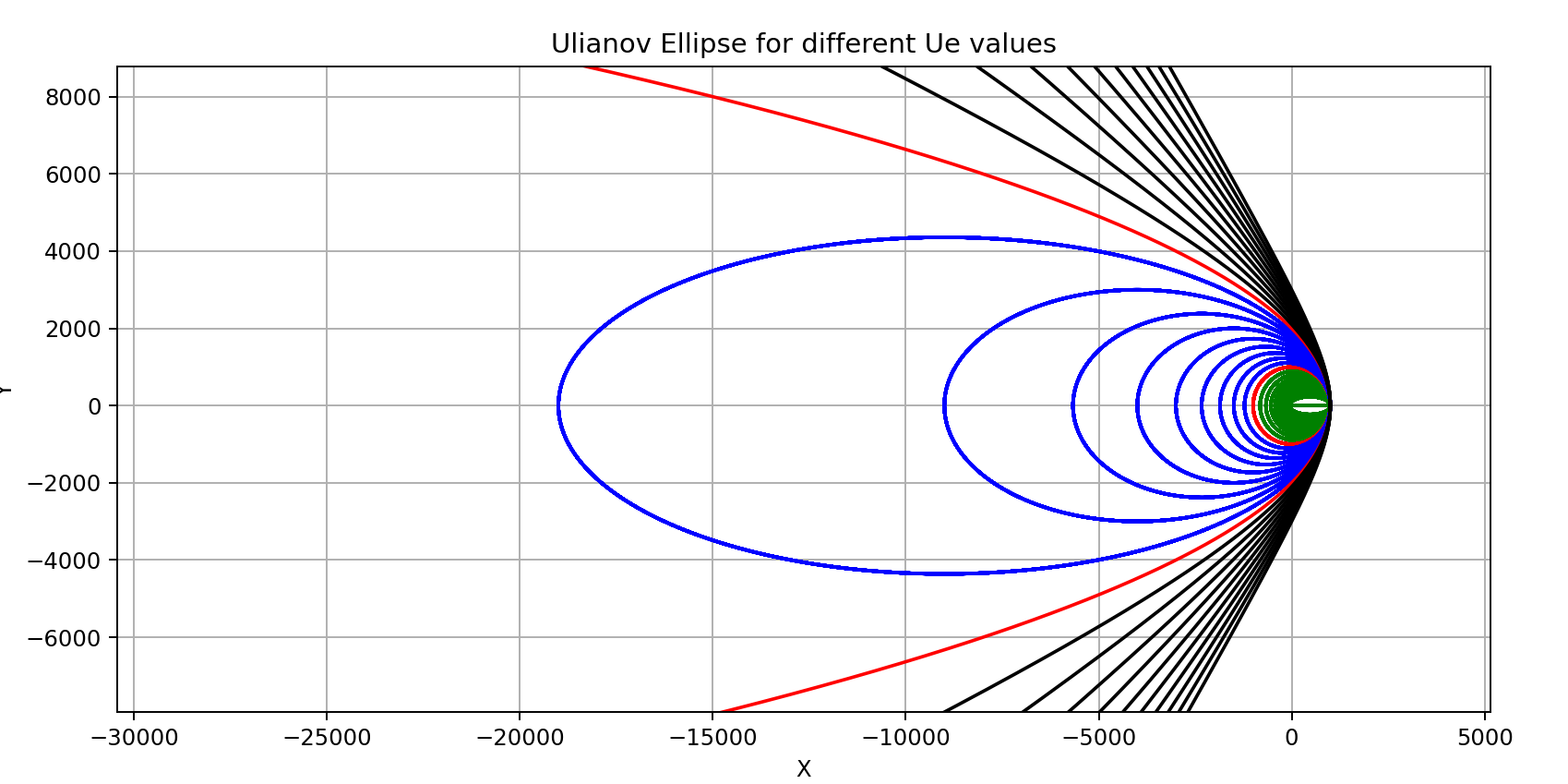
This example showcases the versatility of the ulianovellipse library in visualizing different conic sections, demonstrating the unique properties of the Ulianov Ellipse Parameter.
Example of Use 04: rotateellipses.py
Drawing Incomplete, Bicolor, and Rotated Ellipses
This example illustrates how to use the ulianovellipse library to draw incomplete, bicolor, and rotated ellipses. The functions provided allow for the visualization of various sections of ellipses with different rotations and color schemes.
import numpy as np
import matplotlib.pyplot as plt
from ulianovellipse import eu

def Plot_Two_Ellipses_rotate_degrees_ab(a, b, ang_ellipse=0):
    """
    Plots two ellipses (standard and Ulianov) with given semi-major (a) and semi-minor (b) axes,
    rotated by a specified angle in degrees.

    Parameters:
    a (float): Semi-major axis length.
    b (float): Semi-minor axis length.
    ang_ellipse (float): Rotation angle in degrees for the ellipses.

    The function generates a plot showing both the standard and Ulianov ellipses.
    """
    plt.figure(figsize=(10, 6))
    UE_x, UE_y = eu.ulianov_ellipse_ab(a, b, ang_ellipse_degrees=ang_ellipse)
    SE_x, SE_y = eu.ellipse_ab(a, b, ang_ellipse_degrees=ang_ellipse)
    plt.plot(np.array(SE_x), SE_y, color="red", label='Standard')
    plt.plot(np.array(UE_x), UE_y, color="blue", label='Ulianov')
    plt.legend()
    plt.ylabel("y")
    plt.xlabel("x")
    plt.axis('equal')
    plt.title(f"Ellipses a={a}, b={b}, angle rotate={ang_ellipse}°")
    plt.grid()
    plt.show()

def Plot_Two_Ellipses_rotate_rad_ue(R0, Ue, ang_ellipse=0):
Explanation of the Code
Function Plot_Two_Ellipses_rotate_degrees_ab:
- Description: Plots two ellipses (standard and Ulianov) with given semi-major axis a and semi-minor axis b , rotated by a specified angle in degrees. The ellipses are plotted in different colors to facilitate comparison.
- Parameters:
a: Length of the semi-major axis.b: Length of the semi-minor axis.ang_ellipse: Rotation angle in degrees.
Function Plot_Two_Ellipses_rotate_rad_ue:
- Description: Plots two ellipses (standard and Ulianov) using the parameters R_0 and Ue , rotated by a specified angle in radians. This function is useful for visualizing ellipses with different Ulianov parameters.
- Parameters:
R0: Minimum orbital distance for the Ulianov ellipse.Ue: Ulianov Ellipse Parameter.ang_ellipse: Rotation angle in radians.
Function Plot_Two_Ellipses_incomplete:
- Description: Plots incomplete segments of two ellipses (standard and Ulianov) with semi-major axis a and semi-minor axis b , rotated by a specified angle in degrees. The segments are drawn in different colors, highlighting various parts of the ellipses.
- Parameters:
a: Length of the semi-major axis.b: Length of the semi-minor axis.ang_ellipse: Rotation angle in degrees.
Visualization
The following image demonstrates the output of the three functions with different parameters, highlighting the versatility of the Ulianov elliptical model for creating complex visualizations of ellipses with rotations and incomplete sections.
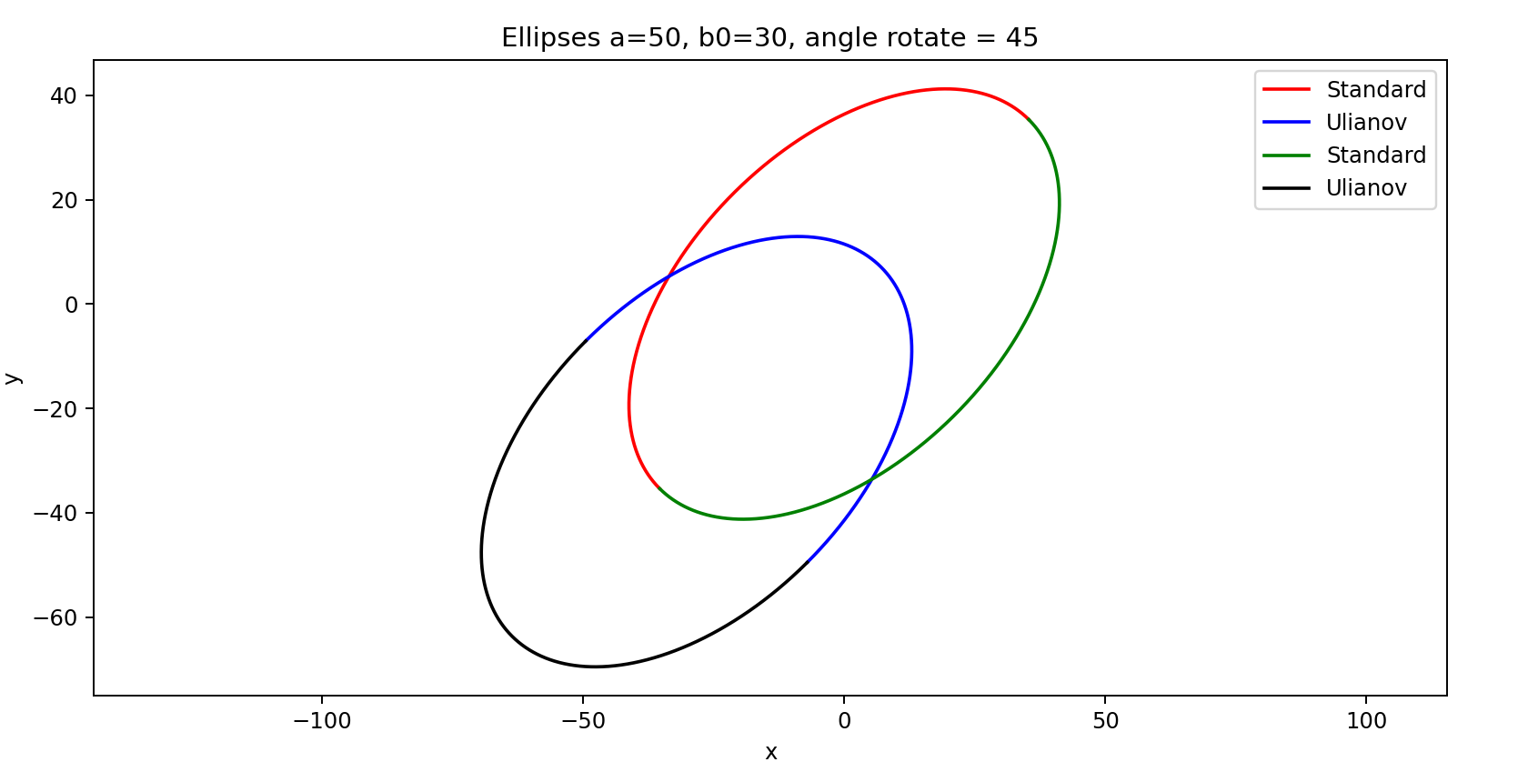
This figure illustrates various elliptical shapes and transformations, showcasing the unique capabilities of the ulianovellipse package for detailed and customizable visualizations.
Example of Use 05: testarctannuell.py
Testing Resolution Errors in the Function arctanuell
The arctanuell function is a key component of the UlianovEllipse library, used to calculate the angle and distance for a given set of coordinates and Ulianov Ellipse parameter Ue . This function is particularly useful in applications where precise calculations of elliptical parameters are required.
Function Definition:
def arctanuell(self, y, x, Ue, precision=1E-10):
    """
    Calculates the Ulianov Ellipse arctangent for a given x and y coordinate and Ue.

    Parameters:
    y (float): Y-coordinate.
    x (float): X-coordinate.
    Ue (float): Ellipse parameter Ue (ranges from 0.500000000000002 to 1.99999999999999).
    precision (float): Desired precision for the calculation.
    msg (int): Verbosity level for debugging messages.

    Returns:
    tuple: (angle, R0)
    angle (float): Calculated angle in radians.
    R0 (float): Calculated R0 value.
    """
    return ang_final, R0n
This function iteratively finds the angle and distance using the x and y coordinates and the Ulianov Ellipse parameter Ue . Due to the iterative nature of the function, there is a rounding error of the order of 10^{-12} % . The accuracy and reliability of the arctanuell function can be tested using a specialized testing routine, as shown below:
Testing Routine:
The test_arctanuell function assesses the accuracy of the arctanuell function by comparing the calculated and original angles and distances for various Ue values.
import numpy as np
import matplotlib.pyplot as plt
from ulianovellipse import eu

def test_arctanuell(lim=0):
    Ue_values = [1.2, 1.5, 1.8, 1.9, 1.95, 1.99, 1.999, 1.9999, 1.99999, 1.999999, 1.99999999, eu.Lim_Ue]
    nump = 5000
    R0 = 10000
    all_alpha = []
    all_error_alpha = []
    all_error_R0 = []

    if lim == 0:
        lim = len(Ue_values)
    if lim > len(Ue_values):
        lim = len(Ue_values)

    for i in range(lim):
        Ue = Ue_values[i]
        print(f"Testing arctanuell for Ue={Ue}")
        alpha = []
        error_alpha = []
        error_R0 = []

        maxerro = 0
        maxerroR0 = 0
        maxct = 0
        mostra = 0

        for t in range(nump):
            ag = (t) * np.pi * 2 / nump
            aggr = ag * 180 / np.pi
            alpha.append(aggr)
            ex = R0 * eu.cosuell(ag, Ue)
            ey = R0 * eu.sinuell(ag, Ue)
            agn, R0n = eu.arctanuell(ey, ex, Ue)
            if eu.last_functon_steps() > maxct:
                maxct = eu.last_functon_steps()
            agngr = agn * 180 / np.pi
            errogr = (agngr - aggr)
            errorR0 = (R0 - R0n) / R0 * 100
            if abs(errogr) > abs(maxerro):
                maxerro = errogr
                angerromax = aggr
            if abs(errorR0) > abs(maxerroR0):
                maxerroR0 = errogr
                angerromaxR0 = aggr
            error_alpha.append(errogr)
            error_R0.append(errorR0)
            mostra += 1
            if mostra > 10:
                mostra = 0
                print(f"\rag gr={aggr:.4f}, agn gr={agngr:.4f}, errogr ={errogr:.6e} ", end="")

        all_alpha.append(alpha)
        all_error_alpha.append(error_alpha)
        all_error_R0.append(error_R0)
        print(f"\nUe={Ue}, Maxerro Alpha= {maxerro} in angle {angerromax}")
        print(f"\nMaxerro R0 = {errorR0} in angle {angerromaxR0}, Max Steps ={maxct}")

    plt.figure(figsize=(10, 6))
    for i in range(lim):
        plt.plot(all_alpha[i], all_error_alpha[i], label=f'Ue={Ue_values[i]}')
    plt.xlabel('Original Alpha')
    plt.ylabel('Error in Alpha (degrees)')
    plt.title(f'arctanuell Alpha Error for Different Ue Values')
    plt.legend()
    plt.grid(True)
    plt.show()

    plt.figure(figsize=(10, 6))
    for i in range(lim):
        plt.plot(all_alpha[i], all_error_R0[i], label=f'Ue={Ue_values[i]}')
    plt.xlabel('Original Alpha')
    plt.ylabel('Error in R0 (%)')
    plt.title(f'arctanuell R0 Error for Different Ue Values')
    plt.legend()
    plt.grid(True)
    plt.show()

# Test the function with a specific number of Ue values
test_arctanuell(4)
Explanation of the Code
The function test_arctanuell is designed to evaluate the accuracy of the arctanuell function from the ulianovellipse library. This function calculates the inverse of the elliptical functions (cosuell and sinuell) for given x and y coordinates, returning the angle ( α ) and distance ( R_0 ).
Parameters:
lim: Limits the number of different Ue values to be tested. If not specified, all values in theUe_valueslist are used.
Core Testing Process:
- Setting up
Uevalues: The function defines a range of Ue values, including values approaching the limiting valueeu.Lim_Ue. - Generating Test Data: For each Ue value, the function generates several points on the ellipse:
exandeycoordinates are calculated using thecosuellandsinuellfunctions for angles from 0 to 360 degrees.- These coordinates are then passed to the
arctanuellfunction, which calculates the corresponding angle ( α ) and distance ( R_0 ).
- Calculating Errors: The differences between the original and calculated angles (
errogr) and the original and calculated distances (errorR0) are computed. - Tracking Maximum Errors: The maximum errors for angle and distance, along with the corresponding angles, are recorded for each Ue .
Visualization: The function generates two plots:
- Error in Alpha: Plots the error in the angle calculation ( α ) against the original angle for different Ue values.
- Error in R_0 : Plots the percentage error in the calculated distance R_0 against the original angle for different Ue values.
These plots help visualize the accuracy and stability of the arctanuell function across a range of Ue values.
Heart of the Test
The central part of the test involves generating multiple positions (ex, ey) for a wide range of angles (0 to 360 degrees) and several Ue values:
ex = R0 * eu.cosuell(ag, Ue)
ey = R0 * eu.sinuell(ag, Ue)
The inverse function arctanuell is then used to recover the angle and distance:
agn, R0n = eu.arctanuell(ey, ex, Ue)
Finally, two types of errors are calculated:
- Error in Angle (degrees):
errogr = (agngr - aggr) - Error in R_0 (percentage):
errorR0 = (R0 - R0n) / R0 * 100
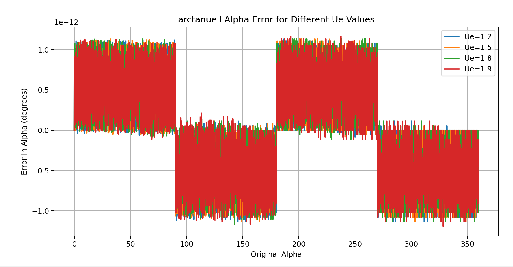
This figure illustrates that the errors in the arctanuell function are in the range of 10^{-12}%. This level of accuracy is impressive and is consistent with the precision limits of the numpy library. To achieve even more precise results, it would be necessary to use libraries like mpmath which allow configurable precision with a large number of decimal places. The next version of the ulianovellipse library plans to include an object named eump that will use mpmath routines instead of numpy, offering precision up to 100 digits.
Example of Use 06: testarctannuellue.py
Testing Resolution Errors in the Function arctanuell_ue
The arctanuell_ue function is a key component of the UlianovEllipse library. It calculates the angle and the Ulianov Ellipse parameter Ue from given x and y coordinates and a reference distance R_0 . This function is essential for accurately determining the properties of an ellipse based on its geometric parameters.
Function Definition:
def arctanuell_ue(self, y, x, R0):
    """
    Calculates the Ulianov Ellipse arctangent and Ue value from R0 value.

    Parameters:
    y (float): Y-coordinate.
    x (float): X-coordinate.
    R0 (float): Ellipse parameter R0.
    Ndig (int): Number of digits for refinement (default is 10).

    Returns:
    tuple: (angle, Ue)
    angle (float): Calculated angle in radians.
    Ue (float): Calculated Ue value (ranges from 0.500000000000002 to 1.99999999999999).
    """
    return angulo, Ue
This function iteratively finds the angle and Ue value using the provided x and y coordinates, along with the reference distance R_0 . Due to the iterative nature of the function, there may be rounding errors. The accuracy and reliability of the arctanuell_ue function can be tested using the following routine:
Testing Routine:
The test_arctanuell_ue function evaluates the accuracy of the arctanuell_ue function by comparing the calculated and original angles and Ue values for various α values.
import numpy as np
import matplotlib.pyplot as plt
from ulianovellipse import eu

def test_arctanuell_ue():
    """
    Tests the accuracy of the arctanuell_ue function across a range of alpha values.

    This function checks the precision of converting between coordinates (x, y) and (alpha, Ue) on the Ulianov ellipse.
    """
    # List of alpha values (in degrees) to test
    alpha_values = [5.12345, 30.1234, 45.12345, 60.12345, 90.12345, 125.12345, 180.12345, 270.12345, 399.12345, 355.12345]
    nump = 100  # Number of points for generating the ellipse
    R0 = 10000  # Reference radius

    all_ue = []  # Store all Ue values tested
    all_error_alpha = []  # Store errors in calculated alpha
    all_error_r0 = []  # Store errors in calculated Ue

    for i in range(len(alpha_values)):
        alpha = alpha_values[i]
        print(f"Testing arctanuell_Ue for alpha={alpha}", end="")
        error_alpha = []  # List to store the angle errors
        error_r0 = []  # List to store the Ue errors
        mat_ue = []  # List to store Ue values for plotting

        maxerro = 0
        maxct = 0
        for j in range(nump):
            Ue = 1 + j * 0.9999999 / nump  # Generate Ue values from 1 to nearly 2
            alpha_rad = alpha * np.pi / 180  # Convert alpha to radians
            print(f"\rTesting arctanuell_Ue for alpha={alpha}, Ue={Ue}", end="")
            mat_ue.append(Ue)

            # Compute the x and y coordinates on the Ulianov ellipse for the given angle and Ue
            xi = R0 * eu.cosuell(alpha_rad, Ue)
            yi = R0 * eu.sinuell(alpha_rad, Ue)

            # Use the arctanuell_ue function to retrieve the angle and Ue from (yi, xi)
            alpha_med, Ue_med = eu.arctanuell_ue(yi, xi, R0)
            if eu.last_functon_steps() > maxct:
                maxct = eu.last_functon_steps()
            alpha_medgr = alpha_med * 180 / np.pi  # Convert the calculated angle to degrees

            # Calculate the error in the calculated angle
            errogr = (alpha - alpha_medgr)
            # Calculate the error in the calculated Ue as a percentage
            errorR0 = (Ue - Ue_med) / Ue * 100

            # Track the maximum errors
            if abs(errogr) > abs(maxerro):
                maxerro = errogr
                uemaxerro = Ue
            error_alpha.append(errogr)
            error_r0.append(errorR0)

        all_ue.append(mat_ue)
        all_error_alpha.append(error_alpha)
        all_error_r0.append(error_r0)
        print(f", Maxerro = {maxerro}, Ue maxerro ={uemaxerro}, Max Steps ={maxct}")

    # Plot the errors in the calculated angles
    plt.figure(figsize=(10, 6))
    for i in range(len(alpha_values)):
        plt.plot(all_ue[i], all_error_alpha[i], label=f'alpha={alpha_values[i]}')
    plt.xlabel('Ue')
    plt.ylabel('Error in Alpha (degrees)')
    plt.title(f'arctanuell Alpha Error for Different Alpha Values')
    plt.legend()
    plt.grid(True)
    plt.show()

    # Plot the errors in the calculated Ue values
    plt.figure(figsize=(10, 6))
    for i in range(len(alpha_values)):
        plt.plot(all_ue[i], all_error_r0[i], label=f'alpha={alpha_values[i]}')
    plt.xlabel('Ue')
    plt.ylabel('Error in Ue (%)')
    plt.title(f'arctanuell Ue Error for Different Alpha Values')
    plt.legend()
    plt.grid(True)
    plt.show()

test_arctanuell_ue()
Explanation of the Code
The test_arctanuell_ue function is designed to evaluate the accuracy of the arctanuell_ue function. This function calculates the inverse of the elliptical functions (cosuell and sinuell) for given x and y coordinates, returning the angle ( α ) and Ulianov Ellipse parameter ( Ue ).
Parameters:
alpha_values: A list of angles in degrees to test the function.nump: Number of points used for generating the ellipse.R0: The reference radius for the ellipse.
Core Testing Process:
- Setting up Ue values: The function defines a range of Ue values, including values close to the limiting value.
- Generating Test Data: For each α value, the function generates several points on the ellipse:
- The coordinates x_i and y_i are calculated using
cosuellandsinuellfor the given angles and Ue values. - These coordinates are then used in the
arctanuell_uefunction to calculate the angle and Ue .
- The coordinates x_i and y_i are calculated using
- Calculating Errors: The differences between the original and calculated angles (
errogr) and the original and calculated Ue values (errorR0) are computed. - Tracking Maximum Errors: The maximum errors for angle and Ue , along with the corresponding angles, are recorded.
Visualization: The function generates two plots:
- Error in Alpha: Plots the error in the angle calculation ( α ) against the calculated Ue values.
- Error in Ue : Plots the percentage error in the calculated Ue values against the original angle for different α values.
These plots provide insights into the accuracy and stability of the arctanuell_ue function across different α and Ue values.
Test Results
The graph produced shows the errors in both alpha and Ue across different test cases, helping to identify any precision issues or inconsistencies in the function's implementation.
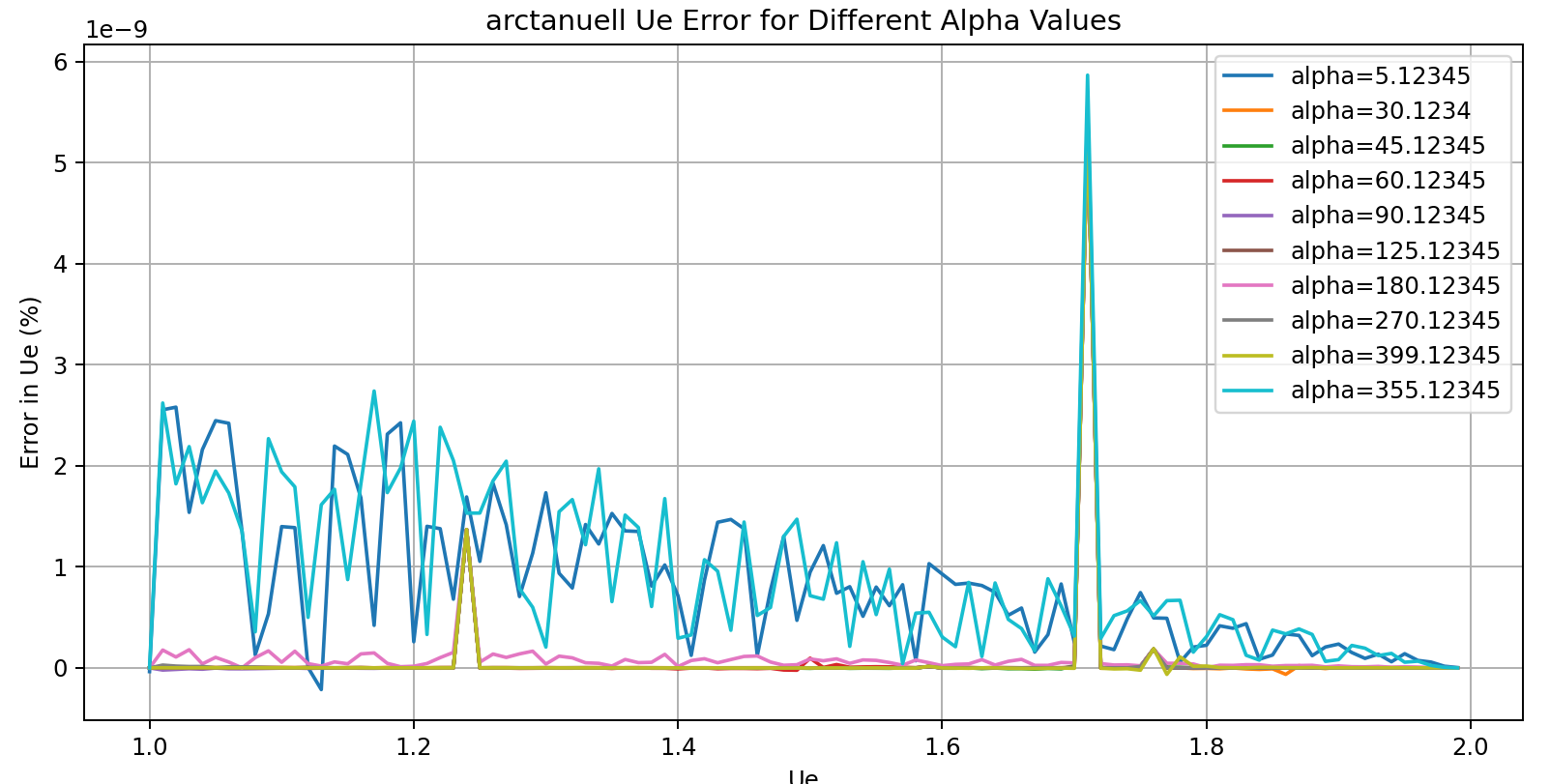
This figure illustrates that the errors in the arctanuell_ue function are in the range of 10^{-9}%. This level of accuracy is impressive and is consistent with the precision limits of the numpy library. To achieve even more precise results, it would be necessary to use libraries like mpmath which allow configurable precision with a large number of decimal places. The next version of the ulianovellipse library plans to include an object named eump that will use mpmath routines instead of numpy, offering precision up to 100 digits.
Example of Use 07: dudaflower.py
The Duda_Flower function creates a flower-like pattern using a combination of standard and Ulianov ellipses. The function accepts various parameters to customize the size, number of petals, colors, and rotation of the flower.
import numpy as np
import matplotlib.pyplot as plt
from ulianovellipse import eu

def Duda_Flower(a, b, ptn=24, gp=0, cla1="green", cla2="red", num_flor_user=0):
    """
    Plots a simplified "Duda Flower" pattern using standard and Ulianov elliptical functions.

    Parameters:
    a (float): Semi-major axis length for the ellipses.
    b (float): Semi-minor axis length for the ellipses.
    ptn (int): Number of petals (default is 24).
    gp (float): Rotation angle in degrees for the petals (default is 0).
    cla1 (str): Color for standard ellipses (default is "green").
    cla2 (str): Color for Ulianov ellipses (default is "red").
    num_flor_user (int): Identifier for the flower pattern (default is 0).

    The function generates a plot of a flower pattern with two layers of ellipses.
    """
    # Ensure a >= b for correct ellipse plotting
    if b > a:
        a, b = b, a

    # Set up the plot
    plt.figure(figsize=(10, 6))

    # First layer with standard ellipses
    for i in range(ptn):
        ang_ellipse = (gp / 180 * np.pi / ptn + (2 * np.pi / ptn * i)) * 180 / np.pi
        SE_x, SE_y = eu.ellipse_ab(a, b, ang_ellipse_degrees=ang_ellipse)
        if cla1 != "none":
            plt.plot(np.array(SE_x), SE_y, color=cla1)

    # Second layer with Ulianov ellipses
    for i in range(ptn):
        ang_ellipse = (gp / 180 * np.pi / ptn + (2 * np.pi / ptn * i)) * 180 / np.pi
        UE_x, UE_y = eu.ulianov_ellipse_ab(a, b, ang_ellipse_degrees=ang_ellipse)
        if cla2 != "none":
            plt.plot(np.array(UE_x), UE_y, color=cla2)

    # Finalize plot settings
    plt.ylabel("y")
    plt.xlabel("x")
    plt.axis('off')
    plt.axis('equal')
    plt.title(f"Duda Flower N$^0${num_flor_user}: a={a},b={b},NP={ptn},G={gp}$^o$,C1={cla1},C2={cla2}")
    plt.savefig(f"DudaFlower{num_flor_user}.jpg")  # Save the plot as an image
    plt.show()

# Example usage with different parameters for each flower
Duda_Flower(a=80, b=60, ptn=36, gp=0, cla1='green', cla2='red', num_flor_user=124)
Duda_Flower(a=240, b=30, ptn=24, gp=180, cla1='red', cla2='blue', num_flor_user=102)
Duda_Flower(a=80, b=30, ptn=24, gp=0, cla1='green', cla2='red', num_flor_user=103)
Duda_Flower(a=50, b=40, ptn=24, gp=0, cla1='green', cla2='blue', num_flor_user=104)
Duda_Flower(a=80, b=30, ptn=24, gp=0, cla1='green', cla2='red', num_flor_user=105)
Duda_Flower(a=240, b=20, ptn=36, gp=180, cla1='green', cla2='red', num_flor_user=177)
Duda_Flower(a=240, b=30, ptn=24, gp=180, cla1='green', cla2='blue', num_flor_user=107)
Duda_Flower(a=80, b=30, ptn=24, gp=180, cla1='green', cla2='red', num_flor_user=108)
Duda_Flower(a=50, b=40, ptn=24, gp=180, cla1='green', cla2='blue', num_flor_user=109)
Duda_Flower(a=80, b=30, ptn=24, gp=180, cla1='green', cla2='blue', num_flor_user=133)
Explanation of the Code
Imports:
numpyandmatplotlib.pyplotare standard libraries for numerical calculations and plotting in Python.euis imported from theulianovellipsepackage, providing functions to compute parameters for the Ulianov ellipse.
Function Duda_Flower:
-
Parameters:
a,b: Semi-major and semi-minor axes of the ellipses.ptn: Number of petals.gp: Rotation angle for the petals.cla1,cla2: Colors for the ellipses.
-
Calculations:
ang_ellipse: Calculated angle for rotating each ellipse.
-
Plotting:
- Ellipses are plotted with specified colors, creating a flower-like pattern.
- The plot includes the title with parameters used to create the flower.
This example demonstrates how to create a complex, visually appealing pattern using both standard and Ulianov ellipses, highlighting the versatility of the ulianovellipse package.
Example of Use 08: saleteflower.py
The Salete_Flower function creates a flower-like pattern using standard and Ulianov ellipses. The function accepts various parameters to customize the size, number of petals, colors, and rotation of the flower.
import numpy as np
import matplotlib.pyplot as plt
from ulianovellipse import eu

def Salete_Flower(a, b, R0, Ue, ptn=24, gp=0, cla1="green", cla2="red", num_flor_user=0):
    """
    Plots a "Salete Flower" pattern using standard elliptical functions for the first layer and Ulianov elliptical functions for the second layer.

    Parameters:
    a (float): Semi-major axis length for the first layer ellipses.
    b (float): Semi-minor axis length for the first layer ellipses.
    R0 (float): Minimum orbital distance for the Ulianov ellipses.
    Ue (float): Ulianov Ellipse Parameter for the Ulianov ellipses.
    ptn (int): Number of petals (default is 24).
    gp (float): Rotation angle in degrees for the petals (default is 0).
    cla1 (str): Color for standard ellipses (default is "green").
    cla2 (str): Color for Ulianov ellipses (default is "red").
    num_flor_user (int): Identifier for the flower pattern (default is 0).

    The function generates a plot of a flower pattern with two layers: one using standard ellipses and the other using Ulianov ellipses.
    """
    # Ensure a >= b for correct ellipse plotting
    if b > a:
        a, b = b, a

    # Set up the plot
    plt.figure(figsize=(10, 6))

    # First layer with standard ellipses
    for i in range(ptn):
        ang_ellipse = (gp / 180 * np.pi / ptn + (2 * np.pi / ptn * i)) * 180 / np.pi
        SE_x, SE_y = eu.ellipse_ab(a, b, ang_ellipse_degrees=ang_ellipse)
        if cla1 != "none":
            plt.plot(np.array(SE_x), SE_y, color=cla1)

    # Second layer with Ulianov ellipses
    for i in range(ptn):
        ang_ellipse = (gp / 180 * np.pi / ptn + (2 * np.pi / ptn * i)) * 180 / np.pi
        UE_x, UE_y = eu.ulianov_ellipse_ue(R0, Ue, ang_ellipse_degrees=ang_ellipse)
        if cla2 != "none":
            plt.plot(np.array(UE_x), UE_y, color=cla2)

    # Finalize plot settings
    plt.ylabel("y")
    plt.xlabel("x")
    plt.axis('off')
    plt.axis('equal')
    plt.title(f"Salete Flower N$^0${num_flor_user}: a={a},b={b},R0={R0},Ue={Ue},NP={ptn},G={gp}$^o$,C1={cla1},C2={cla2}")
    plt.savefig(f"SaleteFlower{num_flor_user}.jpg")  # Save the plot as an image
    plt.show()

# Example usage with different parameters for each flower
Salete_Flower(a=80, b=60, R0=0.268, Ue=1.991, ptn=36, gp=0, cla1='green', cla2='red', num_flor_user=224)
Salete_Flower(a=

240, b=30, R0=2.25, Ue=1.975, ptn=24, gp=180, cla1='red', cla2='blue', num_flor_user=202)
Salete_Flower(a=80, b=30, R0=15.3, Ue=1.745, ptn=24, gp=0, cla1='green', cla2='red', num_flor_user=203)
Salete_Flower(a=50, b=40, R0=23.4, Ue=1.575, ptn=24, gp=0, cla1='green', cla2='red', num_flor_user=204)
Salete_Flower(a=80, b=30, R0=15.3, Ue=1.745, ptn=24, gp=0, cla1='green', cla2='red', num_flor_user=205)
Salete_Flower(a=240, b=20, R0=0.627, Ue=1.992, ptn=36, gp=180, cla1='green', cla2='red', num_flor_user=277)
Salete_Flower(a=240, b=30, R0=2.25, Ue=1.975, ptn=24, gp=180, cla1='green', cla2='red', num_flor_user=207)
Salete_Flower(a=80, b=30, R0=15.3, Ue=1.745, ptn=24, gp=180, cla1='green', cla2='red', num_flor_user=208)
Salete_Flower(a=50, b=40, R0=23.4, Ue=1.575, ptn=24, gp=180, cla1='green', cla2='red', num_flor_user=209)
Salete_Flower(a=80, b=30, R0=15.3, Ue=1.745, ptn=24, gp=180, cla1='green', cla2='red', num_flor_user=233)
Explanation of the Code
Imports:
numpyandmatplotlib.pyplotare standard libraries for numerical calculations and plotting in Python.euis imported from theulianovellipsepackage, providing functions to compute parameters for the Ulianov ellipse.
Function Salete_Flower:
-
Parameters:
a,b: Semi-major and semi-minor axes for the standard ellipses.R0,Ue: Parameters for the Ulianov ellipses.ptn: Number of petals.gp: Rotation angle for the petals.cla1,cla2: Colors for the standard and Ulianov ellipses.
-
Calculations:
ang_ellipse: Calculated angle for rotating each ellipse.
-
Plotting:
- Ellipses are plotted with specified colors, creating a flower-like pattern.
- The plot includes the title with parameters used to create the flower.
Release history Release notifications | RSS feed


Download files
Download the file for your platform. If you're not sure which to choose, learn more about installing packages.
Source Distribution
Built Distribution
Filter files by name, interpreter, ABI, and platform.
If you're not sure about the file name format, learn more about wheel file names.
Copy a direct link to the current filters
File details
Details for the file ulianovellipse-1.8.4.tar.gz.
File metadata
- Download URL: ulianovellipse-1.8.4.tar.gz
- Upload date:
- Size: 1.5 MB
- Tags: Source
- Uploaded using Trusted Publishing? No
- Uploaded via: twine/5.1.1 CPython/3.9.19
File hashes
| Algorithm | Hash digest | |
|---|---|---|
| SHA256 |
2a6f3b4a0f5355d781e29e485a896054eaa1dacec615e7ff95b51e77d7d159cc
|
|
| MD5 |
dd1c239fcdb5e0c865bfe1098f3297f0
|
|
| BLAKE2b-256 |
45c768d92e9bd303335f68ac8dd1a2d92aa8de4ba3edc77cf6397b6575ad6070
|
File details
Details for the file ulianovellipse-1.8.4-py3-none-any.whl.
File metadata
- Download URL: ulianovellipse-1.8.4-py3-none-any.whl
- Upload date:
- Size: 18.5 kB
- Tags: Python 3
- Uploaded using Trusted Publishing? No
- Uploaded via: twine/5.1.1 CPython/3.9.19
File hashes
| Algorithm | Hash digest | |
|---|---|---|
| SHA256 |
42e77fae0aae12710123d4e5b75a943f03b628e58bde377deb6338a16b2bb8af
|
|
| MD5 |
de25aee7698b07be3353869d61e90b04
|
|
| BLAKE2b-256 |
e22a69135db257e2472060dc6aaf7935cc449191d819a9fc5b531d37072f31b5
|






