
Representation adequacy and transport-stability auditing in Python
Verified details
These details have been verified by PyPIProject links
GitHub Statistics
Maintainers

Project description
updatesupport
Are your observed categories good enough for the estimate you are reporting?
updatesupport is a Python library for representation adequacy and
transport-stability auditing. It asks whether a coarse public representation,
such as age band, education band, and sex, is enough to determine an aggregate
estimate once hidden composition inside those public cells is allowed to vary.
The motivating workflow is simple:
- Choose the public categories you would report.
- Choose hidden variables that refine those public categories.
- Choose the target rate or other linear estimand you care about.
- Stress test the estimate while holding the public distribution fixed.
- Report how much the answer could move, which public cells drive the movement, and which extra variables would reduce the ambiguity.
This is useful when a table, dashboard, policy analysis, or model evaluation reports aggregates over coarse categories and you want to know whether those categories are stable enough for the estimate being reported.
Plain-English Example
In the Folktables ACSIncome demo, the public categories are:
AGE_BAND x EDU_BAND x SEX
The hidden variables include occupation, class of worker, weekly-hours band,
race, marital status, birthplace, and relationship status. The observed target
rate is 12.37%: the share of sampled people exceeding the ACSIncome income
threshold.
The stress test keeps the public mix fixed but allows hidden composition inside each public cell to change. Under that stress test, the target rate could range from:
11.79% to 13.44%
The width, 1.65 percentage points, is the transport ambiguity. It means that
hidden composition changes could move the aggregate rate by up to about 1.65
percentage points even when the public demographic mix is held fixed.
That interval is not a confidence interval. It does not measure sampling error. It measures sensitivity to hidden composition under the chosen stress test.
See docs/folktables-acs-income-interpretation.md for the analyst-facing interpretation of this result.
What This Is
updatesupport is an audit layer for finite-state reporting representations. It
helps answer:
- Are the public categories adequate for this estimand?
- If not, how large is the remaining ambiguity?
- Which public cells contribute most to the ambiguity?
- Which hidden variables would make the public representation more stable?
It is not a causal inference package, a sampling-uncertainty estimator, or a replacement for substantive modeling. It can complement those workflows by checking whether the categories used to report an estimate are too coarse.
For causal workflows, use DoWhy, EconML, CausalML, or DoubleML to estimate or
validate causal effects, then use updatesupport to audit whether the public
categories used to report those effects are stable to hidden composition changes.
See docs/causal-library-integration.md.
suite = us.causal_reporting_stability(
    df,
    public=["AGE_BAND", "SEX"],
    hidden=["AGE_BAND", "SEX", "OCC_MAJOR", "WKHP_BAND", "RAC1P"],
    effect="tau_hat",
    weight="sample_weight",
    candidate_refinements=["OCC_MAJOR", "WKHP_BAND", "RAC1P"],
    q=us.q_bounded_shift(0.5),
    sensitivity_min_cell_weights=[10, 25],
    sensitivity_q_presets=[
        "saturated",
        us.q_bounded_shift(0.5),
        "observed",
    ],
    statistical_estimate=ate_hat,
    statistical_interval=(ci_low, ci_high),
    statistical_method="causal estimator bootstrap",
)

print(suite.to_markdown())
Install Locally
uv sync
uv run python -m unittest
For the Folktables examples:
uv sync --extra examples
For the EconML causal example:
uv sync --extra causal
For convex Q presets and custom CVXPY environments:
uv sync --extra cvxpy
For the reproducible benchmark gallery:
uv sync --extra examples --extra causal
For DoWhy CausalRefutation conversion:
uv sync --extra dowhy
Core Model
The library implements a finite-state computational version of the update-relevant support machinery from Update-Relevant Support: Hume's Missing Descent. It models:
- a finite hidden state space
D - a public projection
pi: D -> O - a linear estimand
psi(q) = <h, q> - an admissible environment class
Q, which may be saturated, finite-linear, or convex
The library then checks whether a public or refined support is adequate and quantifies the remaining ambiguity among admissible environments that share the same public law. Simple finite-linear classes use closed-form or linear-program backends; TV, chi-square, KL, Wasserstein, and custom convex restrictions use CVXPY.
Tabular Compiler
Use from_dataframe(...) to compile a pandas-like dataframe or iterable of row
mappings into a finite problem:
import updatesupport as us

grouped = us.from_dataframe(
    rows_or_frame,
    public=["AGE_BAND", "EDU_BAND", "SEX"],
    hidden=["AGE_BAND", "EDU_BAND", "SEX", "OCC_MAJOR", "WKHP_BAND"],
    target="__target__",
    weight="PWGTP",
    min_cell_weight=25,
    q="saturated",
)

interval = grouped.problem.global_transport_modulus()

print(grouped.public_law)
print(interval.lower, interval.upper, interval.diameter)
Each retained hidden cell becomes one finite state. The estimand value for that
state is the weighted empirical target mean inside the cell. The chosen Q
preset fixes the observed public law and then defines which hidden-composition
shifts are admissible: saturated reweighting, bounded linear shifts, or convex
divergence/transport budgets.
Q Presets
Q is the admissible environment class used for the hidden-composition stress
test. The built-in presets are:
q="saturated"orus.q_saturated(): fix the observed public law and allow arbitrary reweighting among retained hidden cells inside each public cell.q=us.q_bounded_shift(radius): fix the observed public law and constrain each hidden-cell mass to stay within(1 +/- radius)times its observed mass.q=us.q_tv_budget(radius): fix the observed public law and constrain total variation distance from the observed hidden distribution. This uses CVXPY.q=us.q_chi_square_budget(radius): fix the observed public law and constrain Pearson chi-square divergence from the observed hidden distribution. This uses CVXPY.q=us.q_kl_budget(radius): fix the observed public law and constrain KL divergence from the observed hidden distribution. This uses CVXPY.q=us.q_wasserstein(cost, radius): fix the observed public law and constrain Wasserstein distance from the observed hidden distribution using an explicit hidden-cell cost matrix. This uses CVXPY.q="observed"orus.q_observed(): use only the observed hidden distribution, giving zero hidden-composition ambiguity.
Install the CVXPY extra before using TV, chi-square, KL, Wasserstein, custom convex environments, or parameterized CVXPY radius sweeps:
uv sync --extra cvxpy
See docs/transport-presets.md for guidance on which preset to use, how to choose radii, and how to interpret sensitivity tables.
Public Descent Report
Use public_descent_report(...) to produce a structured report and render it as
Markdown:
report = us.public_descent_report(
    rows_or_frame,
    public=["AGE_BAND", "EDU_BAND", "SEX"],
    hidden=["AGE_BAND", "EDU_BAND", "SEX", "OCC_MAJOR", "WKHP_BAND"],
    target="__target__",
    weight="PWGTP",
    candidate_refinements=["OCC_MAJOR", "WKHP_BAND"],
    min_cell_weight=25,
    q="saturated",
    title="ACSIncome Representation Adequacy Report",
)

print(report.to_markdown())
The report includes the observed value, stress interval, transport ambiguity, public adequacy flag, worst public fibers, and one-column refinement candidates with before ambiguity, after ambiguity, absolute reduction, and percentage reduction.
Sensitivity Checks
Use sensitivity_report(...) to rerun the audit across Q presets,
min_cell_weight thresholds, and alternative hidden-column sets:
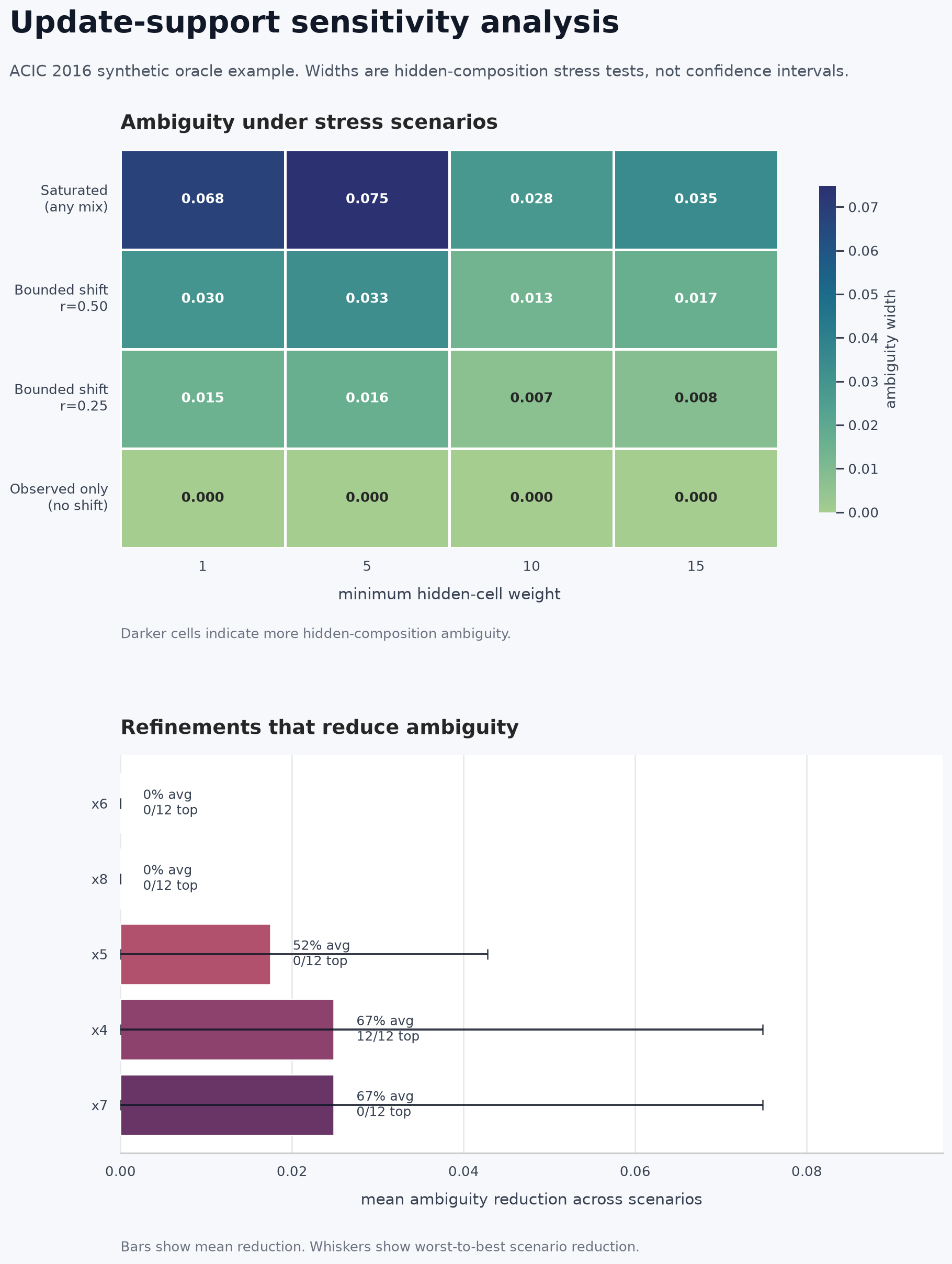
Regenerate the README figure with:
uv run --extra examples python examples/sensitivity_plots.py
sensitivity = us.sensitivity_report(
    rows_or_frame,
    public=["AGE_BAND", "EDU_BAND", "SEX"],
    hidden=["AGE_BAND", "EDU_BAND", "SEX", "OCC_MAJOR", "WKHP_BAND"],
    target="__target__",
    weight="PWGTP",
    min_cell_weights=[1, 10, 25],
    q_presets=["saturated", us.q_bounded_shift(0.5), "observed"],
)

print(sensitivity.to_markdown())
This is the recommended way to check whether the headline ambiguity is sensitive to sparse hidden cells or to the chosen admissible-environment preset. The Markdown output starts with a scenario summary, highlights the lowest- and highest-ambiguity scenarios, flags mixed public-adequacy conclusions, and then renders the full scenario table.
When the grid contains repeated TV, chi-square, KL, or Wasserstein presets that differ only by radius, the sensitivity routines automatically route those rows through the parameterized CVXPY backend and reuse the compiled problem for the fixed hidden state space.
Use recommend_refinements_sensitivity(...) to rank candidate public
refinements across the same kind of grid:
refinements = us.recommend_refinements_sensitivity(
    rows_or_frame,
    public=["AGE_BAND", "EDU_BAND", "SEX"],
    hidden=["AGE_BAND", "EDU_BAND", "SEX", "OCC_MAJOR", "WKHP_BAND", "RAC1P"],
    target="__target__",
    weight="PWGTP",
    candidate_refinements=["OCC_MAJOR", "WKHP_BAND", "RAC1P"],
    min_cell_weights=[1, 10, 25],
    q_presets=["saturated", us.q_bounded_shift(0.5), "observed"],
)

print(refinements.to_markdown())
The aggregate ranking reports mean reduction, worst-case reduction, rank stability, and the number of scenarios where each refinement ranked first.
Public-Fiber-Saturated Example
When all reweightings inside public fibers are admissible, the transport modulus has the closed form:
Omega(p; psi) = sum_o p(o) * (max_{u in pi^-1(o)} h(u) - min_{u in pi^-1(o)} h(u))
import updatesupport as us

problem = us.FiniteProblem(
    states=["a", "b", "c", "d"],
    public={"a": "x", "b": "x", "c": "y", "d": "y"},
    estimand={"a": 0.0, "b": 1.0, "c": 0.0, "d": 3.0},
    environments=us.PublicFiberSaturated(),
)

print(problem.is_public_adequate())
# False

print(problem.fiber_ranges())
# {"x": 1.0, "y": 3.0}

print(problem.global_transport_modulus().diameter)
# 3.0

print(problem.local_transport_modulus({"x": 0.25, "y": 0.75}).diameter)
# 2.5
How To Read A Report
A typical report should separate four ideas:
- Observed value: the estimate under the observed hidden composition.
- Stress interval: the possible estimate range after hidden composition is
varied within the chosen environment class
Q. - Transport ambiguity: the width of that interval.
- Refinement value: how much ambiguity would shrink if another hidden variable were added to the public representation.
The stress interval is a partial-identification or stability interval, not a statistical confidence interval. If the interval is wide, the public categories do not determine the estimate very tightly under the chosen stress test. If the interval is narrow, the estimate is comparatively stable to the modeled hidden composition changes.
Folktables ACS Worked Example
The Folktables example turns ACSIncome or ACSEmployment into an update-support stress test:
- public cells are coarse observed categories such as age band, education band, and sex
- hidden cells refine those categories with occupation, race, work hours, and other task-specific ACS fields
- the estimand is the observed label rate in each hidden cell
- the environment class allows arbitrary reweighting inside the observed public cells while preserving the observed public law
Run the real Folktables ACSIncome example:
uv run --extra examples python examples/folktables_acs.py \
  --task income \
  --states CA \
  --year 2018 \
  --sample 50000 \
  --min-cell-weight 25
Run ACSEmployment instead:
uv run --extra examples python examples/folktables_acs.py \
  --task employment \
  --states CA TX \
  --year 2018
The script prints:
- the observed target rate
- the partial-identification interval under hidden reweighting
- the observed-law transport ambiguity
- a statistical interpretation of the interval and ambiguity
- worst public fibers by ambiguity contribution
- one-column refinements ranked by ambiguity reduction, including before/after ambiguity and percentage reduction
There is also a no-download smoke demo:
uv run python examples/folktables_acs.py --synthetic
There is also a causal-effect reporting example. It fits an EconML CATE
estimator, computes tau_hat = estimator.effect(X), then audits whether that
effect is stable when reported by coarse public categories:
uv run --extra examples --extra causal python examples/folktables_acs_causal.py \
  --task income \
  --states CA \
  --year 2018 \
  --sample 50000
The no-download version is:
uv run --extra causal python examples/folktables_acs_causal.py --synthetic
The built-in first stage uses EconML CausalForestDML. In a real causal
workflow, swap in the DoWhy, EconML, CausalML, or DoubleML estimator that fits
your identification strategy and produces a tau_hat effect target; the
updatesupport stage is the same.
Benchmark Gallery
The benchmark gallery regenerates saved Markdown reports under gitignored
data/benchmark_gallery/:
uv run --extra examples --extra causal python examples/benchmark_gallery.py
It includes no-download Folktables reports plus ACIC 2016 oracle and
EconML-estimated effect reports when data/acic_2016_p1_s1.csv is present. It
also attempts a real Folktables ACS sample from cached data; pass
--folktables-download to fetch the ACS data. See
docs/benchmark-gallery.md.
ACIC 2016 Causal Benchmark Example
The ACIC 2016 example uses the same causal handoff on benchmark-style rows. It
defaults to an oracle effect when potential-outcome columns such as y0/y1 or
mu0/mu1 are present, and otherwise can fit EconML from observed y and z.
The update-support audit defaults to the treated rows, matching the SATT focus
of the 2016 competition. The official assets live in the
vdorie/aciccomp 2016 R package.
Run the no-download smoke demo:
uv run --extra examples python examples/acic_2016.py --synthetic
Run against a CSV exported from the official ACIC 2016 R package:
uv run --extra examples --extra causal python examples/acic_2016.py \
  --input-csv data/acic_2016_p1_s1.csv \
  --effect-source econml \
  --sample 5000
If your exported CSV includes potential outcomes, use --effect-source oracle
and optionally pass --y0-column / --y1-column.
For DoWhy workflows, use audit_dowhy_effects(...) to package the
representation audit with the DoWhy estimate, then call audit.to_refutation()
to produce a DoWhy CausalRefutation object when the optional DoWhy dependency
is installed.
Current Python Surface
Implemented now:
FiniteProblemPartitionPublicFiberSaturatedFiniteEnvironmentsLineSegmentPolytopeEnvironmentsvia SciPylinprogCvxpyEnvironmentsfor convex finite-state environment restrictionsParameterizedCvxpyEnvironmentsfor cached CVXPY radius sweepsfrom_dataframe(...)for compiling grouped tabular data into a finite problem- Q presets:
saturated,observed,bounded_shift,tv_budget,chi_square_budget,kl_budget, andwasserstein PublicDescentReportwith Markdown outputpublic_descent_report(...)for analyst-facing report objectsaudit_effects(...)for causal/uplift effect-reporting stability auditscausal_reporting_stability(...)for packaging causal estimate, statistical uncertainty metadata, hidden-composition ambiguity, sensitivity grids, and public refinement recommendations- estimator adapters:
adapt_dataframe_effects(...),adapt_econml_effects(...),adapt_dowhy_effects(...), andadapt_doubleml_effects(...) audit_dowhy_effects(...)anddowhy_refutation_from_report(...)for DoWhy workflowsrecommend_refinements(...)for ranking candidate hidden variablesrecommend_refinements_sensitivity(...)for aggregating refinement value across Q, hidden-set, and sparsity scenariossensitivity_report(...)for robustness grids over Q, hidden sets, andmin_cell_weightexamples/benchmark_gallery.pyfor regenerating saved Folktables and ACIC benchmark reports under gitignoreddata/benchmark_gallery/- adequacy checks with witnesses
- adequate, minimal, and least support enumeration for small finite problems
- local and global transport moduli
- partial-identification intervals
- cardinal gaps when a least support exists
- simple Markdown reports
Planned next slices:
- experimental transport types such as Gromov-Wasserstein once the comparison object is a pair of relational hidden-state geometries rather than one fixed hidden-cell cost matrix
Finite-Linear Backend
PolytopeEnvironments uses scipy.optimize.linprog for finite-state
environment classes described by linear equality and inequality constraints:
problem = us.FiniteProblem(
    states=["a", "b"],
    public={"a": "o", "b": "o"},
    estimand={"a": 0.0, "b": 4.0},
    environments=us.PolytopeEnvironments(
        constraints=[
            us.geq({"a": 1.0}, 0.25),
            us.geq({"b": 1.0}, 0.25),
        ]
    ),
)

result = problem.global_transport_modulus()

print(result.lower, result.upper, result.diameter)
# 1.0 3.0 2.0
The simplex constraints are implicit. Additional constraints can be supplied
with us.leq(...), us.geq(...), us.eq(...), or us.linear_constraint(...).
Convex CVXPY Backend
CvxpyEnvironments supports the same finite-state simplex and linear
constraints, plus custom convex constraints over the state-probability vector:
def cap_b(_cp, q, _states, state_index):
    return (q[state_index["b"]] <= 0.75,)

problem = us.FiniteProblem(
    states=["a", "b"],
    public={"a": "o", "b": "o"},
    estimand={"a": 0.0, "b": 1.0},
    environments=us.CvxpyEnvironments(
        fixed_public_law={"o": 1.0},
        constraint_builders=(cap_b,),
    ),
)
The TV, chi-square, KL, and Wasserstein Q presets are wrappers around this backend. Use CVXPY when admissible hidden shifts are convex but not just finite-linear constraints.
Solved CVXPY transport intervals expose dual diagnostics:
interval = grouped.problem.global_transport_modulus()
for row in interval.dual_summary(top=5):
    print(row.solve, row.name, row.kind, row.magnitude)
These rows are CVXPY/KKT sensitivity diagnostics. Large multipliers identify
constraints that are locally influential for the solved interval, such as
public-law equalities, Q-budget constraints, or active state lower bounds. Custom
constraint builders can return us.cvxpy_constraint(...) to attach a readable
name and kind to their dual rows.
For repeated radius sweeps on the same compiled finite problem, use the parameterized backend:
grouped = us.from_dataframe(
    rows_or_frame,
    public=["AGE_BAND", "SEX"],
    hidden=["AGE_BAND", "SEX", "OCC_MAJOR"],
    target="__target__",
    q=us.q_tv_budget(0.10, backend="parameterized_cvxpy"),
)

first = grouped.problem.global_transport_modulus()
grouped.problem.environments.set_parameter("radius", 0.20)
second = grouped.problem.global_transport_modulus()
ParameterizedCvxpyEnvironments caches the CVXPY problem and updates CVXPY
parameters for the objective, public law, and preset radius. It is useful when
you are sweeping radii for TV, chi-square, KL, or Wasserstein budgets on a fixed
state space.
Theory Example: No Least Support
The finite poset of adequate supports need not have a least element.
problem = us.FiniteProblem(
    states=["a", "b", "c"],
    public={"a": "o", "b": "o", "c": "o"},
    estimand={"a": 0.0, "b": 1.0, "c": 2.0},
    environments=us.LineSegment(
        center={"a": 1 / 3, "b": 1 / 3, "c": 1 / 3},
        direction={"a": 0.0, "b": 1.0, "c": -1.0},
        radius=1 / 3,
    ),
)

least = problem.least_support()

print(least.exists)
# False

for support in least.minimal_supports:
    print(support.format())
# {{a, c}, {b}}
# {{a, b}, {c}}
More Documentation
Project details
Verified details
These details have been verified by PyPIProject links
GitHub Statistics
Maintainers


Download files
Download the file for your platform. If you're not sure which to choose, learn more about installing packages.
Source Distribution
Built Distribution
Filter files by name, interpreter, ABI, and platform.
If you're not sure about the file name format, learn more about wheel file names.
Copy a direct link to the current filters
File details
Details for the file updatesupport-0.1.0.tar.gz.
File metadata
- Download URL: updatesupport-0.1.0.tar.gz
- Upload date:
- Size: 68.1 kB
- Tags: Source
- Uploaded using Trusted Publishing? Yes
- Uploaded via: twine/6.1.0 CPython/3.13.12
File hashes
| Algorithm | Hash digest | |
|---|---|---|
| SHA256 |
23176172b7f28b30c382e687af05d7adf7bf7fc82963d675d0aff744dfb435af
|
|
| MD5 |
2a59b027cb86acec8899b0ef3fd20053
|
|
| BLAKE2b-256 |
6954c15f66e0720e5c122aeedab7cec74af4a8cec4d490777ee6ab6cf8ae40f3
|
Provenance
The following attestation bundles were made for updatesupport-0.1.0.tar.gz:
Publisher:
publish.yml on nahuaque/updatesupport
-
Statement:
-
Statement type:
https://in-toto.io/Statement/v1 -
Predicate type:
https://docs.pypi.org/attestations/publish/v1 -
Subject name:
updatesupport-0.1.0.tar.gz -
Subject digest:
23176172b7f28b30c382e687af05d7adf7bf7fc82963d675d0aff744dfb435af - Sigstore transparency entry: 2041985122
- Sigstore integration time:
-
Permalink:
nahuaque/updatesupport@74377f8104c83585696e3dcd1c710e06f8c83e60 -
Branch / Tag:
refs/heads/main - Owner: https://github.com/nahuaque
-
Access:
public
-
Token Issuer:
https://token.actions.githubusercontent.com -
Runner Environment:
github-hosted -
Publication workflow:
publish.yml@74377f8104c83585696e3dcd1c710e06f8c83e60 -
Trigger Event:
workflow_dispatch
-
Statement type:
File details
Details for the file updatesupport-0.1.0-py3-none-any.whl.
File metadata
- Download URL: updatesupport-0.1.0-py3-none-any.whl
- Upload date:
- Size: 55.5 kB
- Tags: Python 3
- Uploaded using Trusted Publishing? Yes
- Uploaded via: twine/6.1.0 CPython/3.13.12
File hashes
| Algorithm | Hash digest | |
|---|---|---|
| SHA256 |
f2ced9531003673edcbda51e32425ab146576ce0d0e52330f32a94d767d4ade0
|
|
| MD5 |
168fe3630c3527714d8374d1f19137ab
|
|
| BLAKE2b-256 |
ac9a8f55e38d495c7efbf88a5c3c740b9a168a09b2816d066b882b9f58973c8c
|
Provenance
The following attestation bundles were made for updatesupport-0.1.0-py3-none-any.whl:
Publisher:
publish.yml on nahuaque/updatesupport
-
Statement:
-
Statement type:
https://in-toto.io/Statement/v1 -
Predicate type:
https://docs.pypi.org/attestations/publish/v1 -
Subject name:
updatesupport-0.1.0-py3-none-any.whl -
Subject digest:
f2ced9531003673edcbda51e32425ab146576ce0d0e52330f32a94d767d4ade0 - Sigstore transparency entry: 2041985727
- Sigstore integration time:
-
Permalink:
nahuaque/updatesupport@74377f8104c83585696e3dcd1c710e06f8c83e60 -
Branch / Tag:
refs/heads/main - Owner: https://github.com/nahuaque
-
Access:
public
-
Token Issuer:
https://token.actions.githubusercontent.com -
Runner Environment:
github-hosted -
Publication workflow:
publish.yml@74377f8104c83585696e3dcd1c710e06f8c83e60 -
Trigger Event:
workflow_dispatch
-
Statement type:






