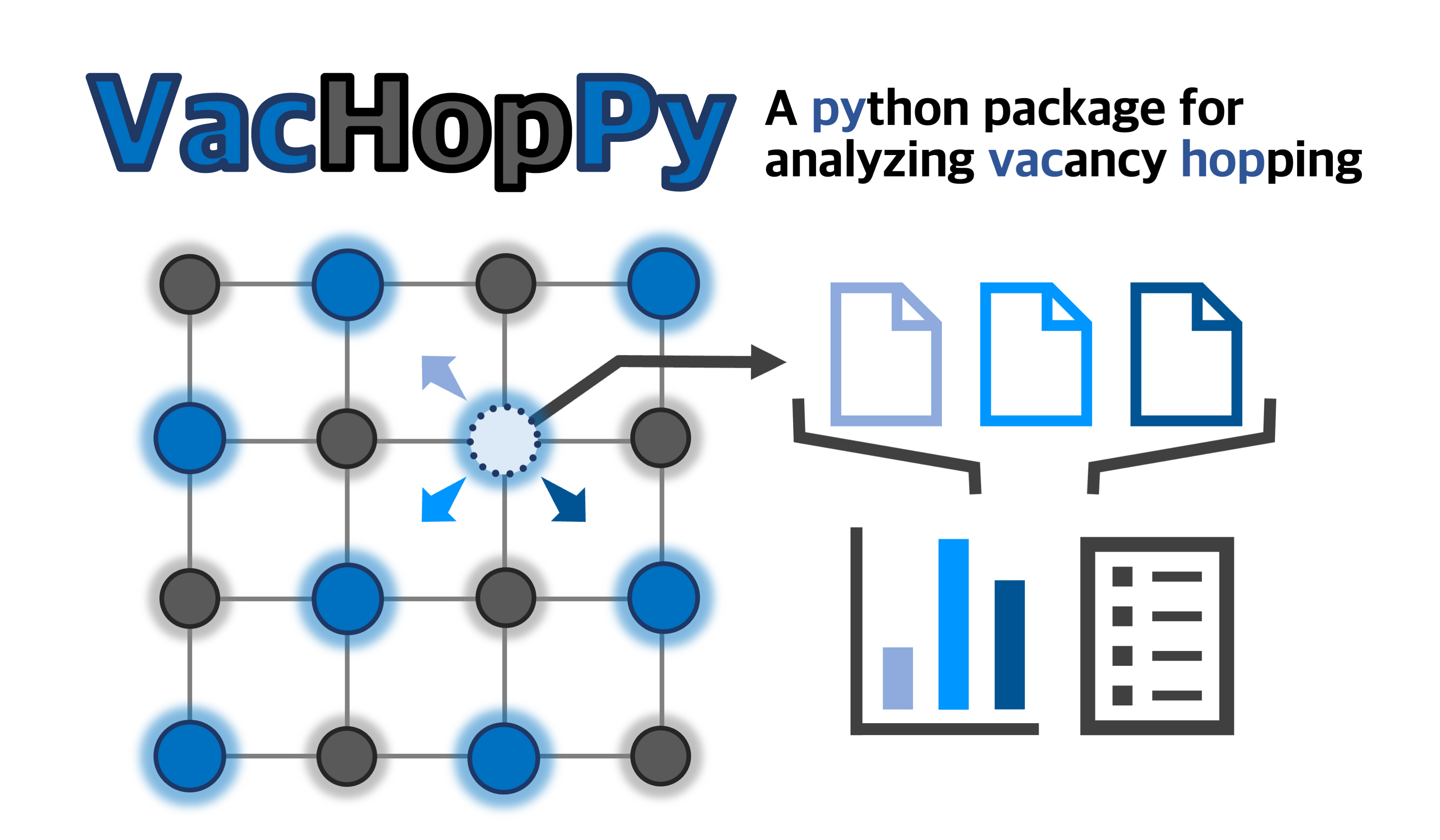
Python package for analyzing vacancy hopping mechanism

Reason this release was yanked:
fix readme.md
Project description
VacHopPy
VacHopPy is a Python package for analyzing vacancy hopping mechanisms based on Ab initio molecular dynamics (AIMD) simulations. A detailed explanation on VacHopPy framwork is available in here.
Features
- Tracking of vacancy trajectories in AIMD simulations
- Extraction of effective hopping parameter set
- Assessment of lattice stability or phase transitions
Effective hopping parameter set, a key improvement of VacHopPy, is a single, representative set of hopping parameters, which is determined by integrating all possible hopping paths in a given system considering energetic and geometric properties. Hence, the effective hopping parameters are suitable for multiscaling modeling, bridging the ab initio calculations and device-scale simulations (e.g., continuum models).
The list of effective hopping parameters, which can be obtained using VacHopPy is summarized below:
| Symbol | Description |
|---|---|
| D | Diffusion coefficient (m²/s) |
| f | Correlation factor |
| τ | Residence time (ps) |
| a | Hopping distance (Å) |
| Eₐ | Hopping barrier (eV) |
| z | Number of equivalent paths |
| ν | Attempt frequency (THz) |
Within the VacHopPy framework, the temperature dependencies of overall diffusion behavior, represented by D and τ, are simplified to an Arrehnius equation composed of the effective hopping parameters. Please see the original paper for a detailed description.
Contents
- Installation
- List of commands
- How to implement
- Preparation
- Vacancy trajectory visualization
- Extraction of effective hopping parameters
- Assessment of lattice stability
- Reference
- License
Installation
This package can be easily installed via pip. The current version of VacHopPy was developed based on VASP 5.4.4.
pip intall vachoppy
If you need parallelized calculations, use:
pip install vachoppy[parallel]
This command automatically download the mpi4py package.
You can download the mpi4py manually:
# for conda environment
conda install mpi4py
# for pip
pip install mpipy
Available commands
VacHopPy provides a command-line interface (CLI). Belows are available CLI commands:
| Option 1 | Option 2 | Use |
|---|---|---|
| -m (main) |
t | Make an animation for vacancy trajectories |
| p | Calculate effective hopping parameters (excluding z and ν) | |
| pp | Calculate z and ν (post-processing for -m p option) | |
| f | Perform fingerprint analyses | |
| -u (utility) |
extract_input | Extract input data (cond.json, pos.npy, force.npy) from vasprun.xml |
| combine_vasprun | Combine two successive vasprun.xml | |
| crop_vasprun | Crop vasprun.xml | |
| fingerprint | Extract fingerprint | |
| cosine_distance | Calculate cosine distance |
For detailed descriptions, please use -h flag:
vachoppy -h # list of available commands
vachoppy -m p -h # explanation for '-m p' mode
For time-consuming commaands, vachoppy -m p and vachoppy -m f, parallelization is supported by mpirun. For parallelization, please specify --parallel option:
vachoppy -m p 0.1 # serial
mpirun -np {num_nodes} vachoppy -m p 0.1 --parallel # parallel
Belows is summary of the main commands (only main modules are shown for clarity):

How to implement
Example files can be downloaded from:
- Example1 : Vacancy hopping in rutile TiO2 download (30 GB)
- Example2 : Phase transition of monoclinic HfO2 at 2200 K download (1.3 GB)
1. Preparation
Input data
To run VacHopPy, the user needs three types of input data: AIMD data, POSCAR_LATTICE, and neb.csv (optional). The current version of VacHopPy supports AIMD simulations performed under the NVT ensemble using VASP only (set MDALGO = 2). Integration with LAMMPS will be supported in the next release.
(1) AIMD data
AIMD data can be extracted from the vasprun.xml file (a standard VASP output) using the following command:
vachoppy -u extract_int -v vasprun.xml
# -v flag is optional (default: vaspun.xml)
This command generates three files: cond.json, pos.npy, and force.npy. Descriptions of each file are provided below:
-
cond.json
cond.json contains simulation conditions, such as temperature, time, atom numbers, and lattice parameters. -
pos.npy (numpy binary)
pos.npy contains evolution in atomic positions during the simulation. The raw trajectories are refined with consideration of periodic boundary condition (PBC). -
force.npy (numpy binary)
force.npy contains force vectors acting on atoms.
(2) POSCAR_LATTICE
This file contains the perfect crystal structure without vacnacies. Its lattice parameters must match those of input structure (POSCAR) of the AIMD simulations. This file is used to define the lattice points for vacancy identification.
(3) neb.csv (optional)
This file contains hopping barriers (Eₐ) for all vacancy hopping paths in the system. Below is an example of neb.csv (example system: rutile TiO2):
# neb.csv
A1,0.8698
A2,1.058
A3,1.766
Here, the first column corresponds to the path names, and the second column contains the Eₐ values. The user can obtain a list of possible vacancy hopping paths by running the vachoppy -m t or vachoppy -m p command. For the vachoppy -m t command (used with the -v flag), hopping path information is saved to the trajectory.txt file. For the vachoppy -m p command, the information is saved to the parameter.txt file.
Note1: the neb.csv file is only required to extract the effective values for coordination number (z) and attempt frequency (ν) (by running the
vachoppy -m ppcommand).
Note2: It is highly recommended to perform NEB calculations using a larger supercell than that used in AIMD simulations. In AIMD, thermal fluctuations attenuate interactions with periodic images and provide a broader sampling of atomic configurations, which helps approximate the effects of a larger supercell.
(4) File organization
Since AIMD simulations commonly cover timescales shorter than nanoseconds, a single AIMD simulation may contain a few hopping events. However, since VacHopPy computes the effective hopping parameters in static manner, sufficient sampling of hopping events is necessary to ensure reliablilty. To address this, VacHopPy processes multiple AIMD datasets simultaneously. Each AIMD dataset is distinguished by a label appended after an underscore in the file names (e.g., cond_{label}.json, pos_{label}.npy, force_{label}.npy). Below is an example of the recommended file structure:
Example1
 ┣ traj # name (traj) is specified by -p1 flag
 ┃ ┣ traj.1900K # prefix (traj) is specifed by -p2 flag
 ┃ ┃ ┣ cond_01.json, pos_01.npy, force_03.npy
 ┃ ┃ ┣ cond_02.json, pos_02.npy, force_03.npy
 ┃ ┃ ┗ cond_02.json, pos_02.npy, force_04.npy
 ┃ ┣ traj.2000K
 ┃ ┃ ┣ cond_01.json, pos_01.npy, force_03.npy
 ┃ ┃ ┣ cond_02.json, pos_02.npy, force_03.npy
 ┃ ┃ ┗ cond_02.json, pos_02.npy, force_04.npy
 ┃ ┗ traj.2100K
 ┃   ┣ cond_01.json, pos_01.npy, force_03.npy
 ┃   ┣ cond_02.json, pos_02.npy, force_03.npy
 ┃   ┗ cond_02.json, pos_02.npy, force_04.npy
 ┃
 ┣ POSCAR_LATTICE
 ┗ neb.csv
The name of the outer directory is specified by the -p1 flag (default: traj), and the prefix of the inner directories is specified by the -p2 flag (default: traj). Each inner directory must contain AIMD datasets generated at the same temperature.
Hyperparameter: tinterval
To run VacHopPy, the user needs to determine one hyperparameter, tinterval, in advance. This parameter defines the time interval for averaging atomic positions and forces. Thermal fluctuations in AIMD simulations can obscure precise atomic occupancy determination. However, since these fluctuations are random, they can be effectively averaged out over time. VacHopPy processes AIMD data by dividing it into segments of length of tinterval. Each segment represents a single step in the analysis. The total number of steps is given by tsimulation/tinterval, where tsimulation is the total AIMD simulation time.

Choosing an appropriate tinterval is crucial for reliable analysis. The tinterval should be large enough to mitigate thermal fluctuations but short enough to prevent multiple hopping events from being included in a single step. A typical value is around 0.05-0.1 ps, through it may vary depending on the system.
One recommended approach for determining the optimal tinterval is through convergence tests using the correlation factor (f). Below is an example of a convergence test (example system: rutile TiO2):

The left and rigut figures show the convergences of f with respect to the number of AIMD datasets (Ncell) and tinterval, respectively, at each temperature. The results confirm that convergence is achieved at Ncell=20 and tinterval=0.07 ps.
2. Vacancy trajectory visualization
Download Example1 directory linked above.
Navigate to the Example1 directory and run:
 vachoppy -m t 0.07 2100 07 -v
 # t_interval, temperature, label
Here, the arguments are:
- tinterval = 0.07 ps
- temperature = 2100 K
- label = 07
The -v flag (verbosity flag) enables the generation of the trajectory.txt file, which contains the identified vacancy hopping paths and hopping history. You can adjust the resolution of the animation using the --dpi option (default: 300). The number and type of vacancies are automatically determined by comparing the POSCAR_LATTICE file with the AIMD datasets.
Output:
The trajectory animation is saved as traj.gif, with individual snapshots stored in the snapshot directory. Below is an example of traj.gif:

In this animation, the solid box represents the lattice (here, rutile TiO2 2×2×3 supercell), and the color-coded circles indicate the lattice points corresponding to the selected atom type (here, oxygen). The yellow-colored circles mark the vacancy positions, while other colors denote occupied lattice points. Atomic movements are depicted with arrows matching the color of the moving atoms.
Occasionally, spurious vacancies may appear; hence, the detected number of vacancies exceeds the initial count in the system. This scenario arise when two or more atoms are assigned to the same lattice site and are commonly associated with non-vacancy-hopping mechanism (e.g., kick-out mechanism). Since such spurious vacancies commonly disappear within a few hundred femtoseconds, they are termed transient vacancies.
In this animation, the transient vacancies are represented as orange-colored circles. Below three successive snapshots shows the kick-out mechanism:

3. Extraction of effective hopping parameters
Navigate to the Example1 directory and run:
# For serial computation
vachoppy -m p 0.07 # t_interval

# For parallel computation
mpirun -np {num_nodes} vachoppy -m p 0.07 --parallel
Here, the arguments are:
- tinterval = 0.1 ps
For serial computation, the process is displayed via a progress bar. For parallel computation, process is recorded in the VACHOPPY_PROGRESS file in real time. The number and type of vacancies are automatically determined by comparing the POSCAR_LATTICE file with the AIMD datasets.
Output:
All results are stored in parameter.txt file, which includes:
- A list of vacancy hopping paths in the system
- Effective hopping parameters (except for z and ν)
- Vacancy hopping history for each AIMD dataset.
To print the vacancy hopping paths, use:
awk '/Vacancy hopping paths :/ {f=1} f; /^$/ {f=0}' parameter.txt
To pring the effective hopping parameters, use:
awk '/Effective/ {f=1} f; /^$/ {f=0}' parameter.txt
3-1. Extract effective values for z and ν (optional)
To obtain the effective values of z and ν, users must first perform NEB calculations for all vacancy hopping paths. The results of the NEB calculations should be stored in a file named neb.csv (see above).
Navigate to the Example1 directory and run:
vachoppy -m pp
This command reads parameter.txt and neb.csv files and outputs postprocess.txt which contains the complete set of the effective hopping parameters.
To print the effective hopping parameters, use:
awk '/hopping parameter/ {f=1} f; /^$/ {f=0}' postprocess.txt
Below is the expected output:

Additionally, VacHopPy provides individual attempt frequencies for each hopping path. To print them, use
awk '/Jump attempt frequency/ {f=1} f; /^$/ {f=0}' postprocess.txt
Attempt frequencies are estimated based on statistical approach. Therefore, only the values for hopping paths with a sufficient number of hopping events can be considered reliable.
4. Assessment of lattice stability
Download and unzip the Example2 file linked above.
VacHopPy employs the fingerprint analysis proposed by Oganov et al. to assess lattice stability. The key quantities used in this analysis are the fingerprint vector (ψ) and the cosine distance (dcos). Detailed descriptions can be found in this paper.
Fingerprint vector (ψ)
To construct ψ, three parameters are required:
- Threshold radius (Rmax)
- Bin size (Δ)
- Standard deviation for Gaussian-smeared delta function (σ)
A well-defined ψ satisfies ψ(r=0) = -1 and converges to 0 as r → ∞. Therefore, the user needs to set these parameters appropriately to ensure these conditions are met. The ψ can be generated by using vachoppy -u fingerprint command:
Navigate to the Example2 directory and run:
vachoppy -u fingerprint POSCAR_MONO 20.0 0.04 0.04 -d
# POSCAR_REF, R_max, Δ, σ
Here, the arguments are:
- Atomic structure = POSCAR_MONO (monoclinic HfO2)
- Rmax = 20 Å
- Δ =0.04 Å
- σ = 0.04 Å
Using -d flag displays the resulting ψ in a pop-up window. Below is an example output (ψ for monoclinic HfO2):

To enhance robustness of ψ, VacHopPy considers all possible atom pairs (e.g., Hf-Hf, Hf-O, and O-O) and concatenates them to construct a single well-defined ψ.
Cosine distance (dcos)
Cosine distance (dcos(x)) quantifies structural similarity to a reference phase x, where a lower dcos(x) indicates a greater similarity. By analyzing variations in dcos(x) over time, users can assess lattice stability or explore phase transitions occurred in the AIMD simulations.
(1) Assessment of lattice stability
Navigate to the Example2 directory and run:
# For serial computation
vachoppy -m f 0.07 20 0.04 0.04 -v vasprun_1600K.xml -p POSCAR_MONO

# For parallel computation
mpirun -np {num_nodes} vachoppy -m f 0.07 20 0.04 0.04 -v vasprun_1600K.xml -p POSCAR_MONO --parallel
Here, the arguments are:
- tinterval = 0.07 ps
- Rmax = 20 Å
- Δ = 0.04 Å
- σ = 0.04 Å
The -v flag specifies vasprun.xml file (default: vasprun.xml), where vasprun_1600K.xml contains the AIMD trajectory at 1600 K. The -p flag specifies the reference phase (default: POSCAR_REF), where POSCAR_MONO contains monoclinic HfO2 lattice.
Results are stored in cosine_distance.txt and cosine_distance.png. To prevent overwriting, rename cosine_distance.txt to dcos_1600K_mono.txt.
Next, run:
# For serial computation
vachoppy -m f 0.07 20 0.04 0.04 -v vasprun_2200K.xml -p POSCAR_MONO

# For parallel computation
mpirun -np {num_nodes} vachoppy -m f 0.07 20 0.04 0.04 -v vasprun_2200K.xml -p POSCAR_MONO --parallel
Here, vasprun_2200K.xml contains the AIMD data at 2200 K. Rename cosine_distance.txt to dcos_2200K_mono.txt.
For comparison, plot dcos_1600K_mono.txt and dcos_2200K_mono.txt together using plot.py:
# plot.py
import sys
import numpy as np
import matplotlib.pyplot as plt

data, num_data = [], len(sys.argv)-1
for i in range(num_data):
    data.append(np.loadtxt(sys.argv[i+1], skiprows=2))

plt.rcParams['figure.figsize'] = (6, 2.5)
plt.rcParams['font.size'] = 10

space = 0.09
for i, data_i in enumerate(data):
    data_i[:,1] -= np.average(data_i[:,1]) - space * i
    plt.scatter(data_i[:,0], data_i[:,1], s=10)

plt.yticks([])
plt.xlabel('Time (ps)', fontsize=12)
plt.ylabel(r'$d_{cos}$($x$)', fontsize=12)
plt.legend(loc='center right')
plt.show()
python plot.py dcos_1600K_mono.txt dcos_2200K_mono.txt

In this figure, the dcos data at each temperature is arranged vertically; hence, the absolute y-values are meaningless. Instead, the focus is on the relative change in dcos over time.
- At 1600 K, dcos remains nearly constant, indicating structural stability.
- At 2200 K, dcos exhibits substantial fluctuations near 20 ps, suggesting that the monoclinic lattice becomes unstable at high temperatures.
It is important to note that the lattice parameters were contrained to those of monoclinic lattice since the AIMD simulations were performed under NVT ensmeble. As a result, any lattice distortion is not sustained but instead revert to the original lattice, producing peaks in the dcos trace.
In unstable lattices, such as monoclinic HfO2 at 2200 K, vacancies are poorly defined since atomic vibrtaion centers may shift away from the original lattice point. Consequently, vacancy trajectory determination (vachoppy -m t) and effective hopping parameter extraction (vachoppy -m p) may lack accuracy.
(2) Exploring phase transition
By varying the reference phase, users can explore phase transitions occuring in AIMD simulatoins.
Navigate to the Example2 directory and run:
# For serial computation
vachoppy -m f 0.07 20 0.04 0.04 -v vasprun_2200K.xml -p POSCAR_TET

# For parallel computation
mpirun -np {num_nodes} vachoppy -m f 0.07 20 0.04 0.04 -v vasprun_2200K.xml -p POSCAR_TET --parallel
Here, POSCAR_TET contains the atomic structure of tetragonal HfO2. To prevent overwriting, rename cosine_distance.txt to dcos_2200K_tet.txt.
Next, run:
# For serial computation
vachoppy -m f 0.07 20 0.04 0.04 -v vasprun_2200K.xml -p POSCAR_AO

# For parallel computation
mpirun -np {num_nodes} vachoppy -m f 0.07 20 0.04 0.04 -v vasprun_2200K.xml -p POSCAR_AO --parallel
Here, POSCAR_AO contains the atomic structure of antipolar orthorhombic HfO2. Rename cosine_distance.txt to dcos_2200K_ao.txt.
To compare the results, run plot.py:
python plot.py dcos_2200K_mono.txt dcos_2200K_tet.txt dcos_2200K_ao.txt

As before, the dcos data is arranged vertically, so the absolute y-values are not meaningful. Instead, the focus is on the relative change in dcos over time.
- As dcos(mono) increases,
- dcos(tet) decreases,
- while dcos(ao) remain nearly constant.
This result clearly suggets that the phase transition is directed toward the tetragonal phase.
Reference
If you used VacHopPy package, please cite this paper
If you used vachoppy -m f or vachoppy -u fingerprint commands, also cite this paper.
Release history Release notifications | RSS feed


Download files
Download the file for your platform. If you're not sure which to choose, learn more about installing packages.
Source Distribution
Built Distribution
Filter files by name, interpreter, ABI, and platform.
If you're not sure about the file name format, learn more about wheel file names.
Copy a direct link to the current filters
File details
Details for the file vachoppy-1.0.0.tar.gz.
File metadata
- Download URL: vachoppy-1.0.0.tar.gz
- Upload date:
- Size: 61.1 kB
- Tags: Source
- Uploaded using Trusted Publishing? No
- Uploaded via: twine/6.1.0 CPython/3.10.13
File hashes
| Algorithm | Hash digest | |
|---|---|---|
| SHA256 |
72ffed590198fad61f406fd6a797f897524ff564a61cfd87d383c8ab5498d578
|
|
| MD5 |
f514b487349e920a55156cecec27fae1
|
|
| BLAKE2b-256 |
b7fe092e5aa9d2d624b4f6c34ea66e37c486e3eabdfd4a5b76524641efc74330
|
File details
Details for the file vachoppy-1.0.0-py3-none-any.whl.
File metadata
- Download URL: vachoppy-1.0.0-py3-none-any.whl
- Upload date:
- Size: 58.1 kB
- Tags: Python 3
- Uploaded using Trusted Publishing? No
- Uploaded via: twine/6.1.0 CPython/3.10.13
File hashes
| Algorithm | Hash digest | |
|---|---|---|
| SHA256 |
2cd656b9d06c3029586bbe24ec1cbbaa9845450350fe837764b938b9689ca7df
|
|
| MD5 |
8a01c532910c0b3ebe127c5c2e37a8fc
|
|
| BLAKE2b-256 |
b5f6183d02dd297e60681c920cf8e051306ef9da93873132f0fae7919ec602d5
|


