
velocileptors
Velocity-based perturbation theory (both Lagrangian (LPT) and Eulerian (EPT) formulations) expansions of redshift-space distortions and velocity statistics.
This code computes the real- and redshift-space power spectra and correlation functions of biased tracers using 1-loop perturbation theory (with effective field theory counter terms and up to cubic biasing) as well as the real-space pairwise velocity moments.
The code can be installed with
python3 -m pip install -v git+https://github.com/sfschen/velocileptors
It requires numpy, scipy and pyFFTW (the python wrapper for FFTW):
https://hgomersall.github.io/pyFFTW/
to run. Note that pyFFTW is pip and conda installable and available from conda-forge (we have found the conda-forge channel to be the most reliable).
An example calculation to reproduce the plots in the paper is given in "Moment Expansion Example.ipynb". A short notebook detailing the same steps for the Fourier Streaming Model is given in "Fourier Streaming Model Example.ipynb". Also included is "Gaussian Streaming Model Example.ipynb" that runs through how to produce the correlation function multipoles. An example of the most common use-cases is given in "lpt_examples.py" and more detailed examples of the LPT and EPT power spectrum calculations are given in the appropiately named notebooks. We expect most users will want to use either the lpt_rsd or ept_fullresum models, described in some detail in the "Direct LPT RSD Examples" and "EPT Examples" notebooks.
For most situations computing the power spectrum wedges or multipoles is as simple as:
from velocileptors.LPT.moment_expansion_fftw import MomentExpansion

mome        = MomentExpansion(klin,pklin,threads=nthreads)
kw,pkw      = mome.compute_redshift_space_power_at_mu(pars,f,mu,reduced=True)
kl,p0,p2,p4 = mome.compute_redshift_space_power_multipoles(pars,f,reduced=True)
The core rsd modules are distributed into two directories, one for the LPT theory and one for the EPT theory (plus supporting routines in the Utils directory). Running the EPT version of the above simply requires substituting the "LPT" for "EPT" in the import statement, though can be made more robust by supplying a cosmology-conscious no-wiggle power spectrum via the keyword pnw. See the READMEs in those directories and the example notebooks for more information and examples.
For the most common case of computing the redshift-space power spectrum one can use a a reduced set of parameters and beyond_gauss=False:
pars = [b1, b2, bs, b3] + [alpha0, alpha2, alpha4] + [sn, sn2]
where
(1) b1, b2, bs, b3: the bias parameters up to cubic order
(2) alpha0, alpha2, alpha4: counter terms of the form mu^n.
(3) sn, sn2: stochastic contributions to P_real(k), sigma^2 [e.g. shot-noise, finger-of-god dispersion and kappa].
To include higher order terms in the moment expansion set beyond_gauss=True. In this case you need to additionally specify an alpha6 counterterm and an sn4 stochastic term.
You can also set the AP parameters using keywords apar and aperp.
If you additionally want access to the velocity statistics, then the full set of parameters is
pars = [b1, b2, bs, b3] + [alpha, alpha_v, alpha_s0, alpha_s2, alpha_g1, alpha_g3, alpha_k2] + [sn, sv, s0, s4]
where the parameters are:
(1) b1, b2, bs, b3: the bias parameters up to cubic order
(2) alpha, alpha_v, alpha_s0, alpha_s2, alpha_g1, alpha_g3, alpha_k2: the one-loop counterterms for each velocity component
(3) sn, sv, s0, s4: the stochastic contributions to the velocities
Again, for most practical purposes one can set beyond_gauss=False, in which case the code only uses up to sigma(k), and uses a counterterm ansatz for the third and fourth moments. In this case the parameters alpha_g1, alpha_g3, alpha_k2, and s4 are not used.
More details can be found in Chen, Vlah & White (2020), https://arxiv.org/abs/2005.00523 and Chen, Vlah, Castorina & White (2020), https://arxiv.org/abs/2012.04636
In addition to the above there are two "direct expansion" modules available in LPT and EPT. These are LPT.lpt_rsd_fftw and EPT.ept_fullresum_fftw. The former is described in arXiv:2012.04636 while the latter is described in the original velocileptors paper (arXiv:2005.00523). Both these models take the full bias vector
pars = [b1, b2, bs, b3] + [alpha0, alpha2, alpha4, alpha6] + [sn, sn2, sn4]
The LPT module has to be called slightly differently compared to the other ones because the angular dependence of the underlying IR resummation requires recomputing the PT integrals at each mu. For example the multipoles can be computed as:
from velocileptors.LPT.lpt_rsd_fftw import LPT_RSD
lpt = LPT_RSD(klin,plin,kIR=0.2)

lpt.make_pltable(f,nmax=4,apar=1,aperp=1)
kl,p0,p2,p4 = lpt.combine_bias_terms_pkell(pars)
Further calls, for example for wedges P(k,mu), can be found in the example notebooks.
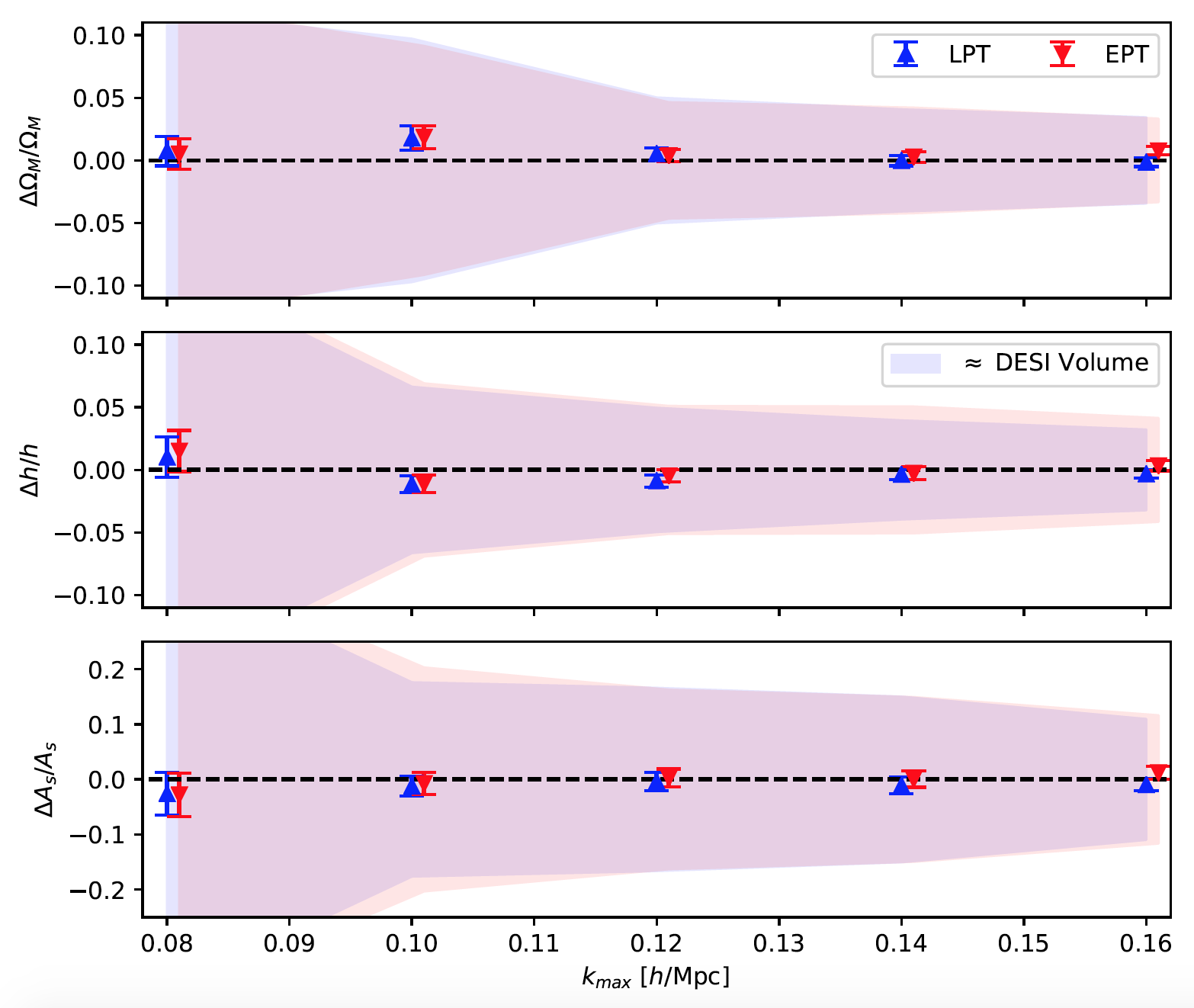
The velocileptors code was entered into the blind mock challenge described here. We summarize the results in the figure below, where the shaded regions are errors for a 5 (Gpc/h)^3 volume with the same signal.
This code is related to the configuration-space based code https://github.com/martinjameswhite/CLEFT_GSM.
Much of the structure of this code is based on the earlier LPT code by Chirag Modi:
https://github.com/modichirag/CLEFT
which used the the mcfit class:
https://github.com/eelregit/mcfit
The main modification is that we save the Mellin transform kernels used in FFTLog to save time, since they take more time than the fft's themselves to evaluate.
We thank Arnaud De Mattia for help debugging features involving massive neutrinos.


Release files for velocileptors 3.1
For a detailed explanation of source distributions (sdists) and built distributions (wheels), please see the package formats documentation.
Source distribution (sdist)
| File | Size | Uploaded | |
|---|---|---|---|
| velocileptors-3.1.tar.gz | 52.1 kB | Details |
Built distribution (wheel)
| File | Interpreter | ABI | Platform | Reset |
|---|---|---|---|---|
| velocileptors-3.1-py3-none-any.whl | Python 3 | none | any | Details |
Total release size: 122.0 kB
Release files / velocileptors-3.1.tar.gz
| Download URL | velocileptors-3.1.tar.gz |
|---|---|
| Size | 52.1 kB |
| Tags | Source |
|
SHA-256 checksum How to use checksums |
2f218e5effeda665c87887171f81e9d01bb5071ebdff06bc9532cce98f117f28
|
|
BLAKE2b-256 checksum How to use checksums |
7f455dca42b30644989f64368e47877f618ed8f1f380a7f6e4b4e955a867bfe7
|
| Upload date | |
|
Uploaded using Trusted Publishing? What is trusted publishing? |
No |
| Uploaded via |
twine/6.2.0 CPython/3.11.13
|
Release files / velocileptors-3.1-py3-none-any.whl
| Download URL | velocileptors-3.1-py3-none-any.whl |
|---|---|
| Size | 69.9 kB |
| Tags | Python 3 |
|
SHA-256 checksum How to use checksums |
c4718fd624a6ec78d2db20543f8e2f05262316c34554bbfbeef7b0a41767b77a
|
|
BLAKE2b-256 checksum How to use checksums |
dbb0213e843d75931a8f684596b49e949474be0933b69e8b5b21cbd071560ae6
|
| Upload date | |
|
Uploaded using Trusted Publishing? What is trusted publishing? |
No |
| Uploaded via |
twine/6.2.0 CPython/3.11.13
|














