
ViewGraphForge




ViewGraphForge generates view graphs for the global stage of Structure-from-Motion (SfM) and evaluates solvers on them: rotation averaging, translation averaging, SE(3) pose-graph optimisation and the detection of outlier edges. It is the generator of ViewGraphBench, a dataset of 45,495 view graphs with 12 to 100,000 cameras each.
A graph is made by simulating the front end of a global-SfM pipeline on a procedural 3-D scene. Cameras following one of seven capture patterns observe the scene points; edges come from co-visibility and an image-retrieval step; match counts and measurement errors follow from the viewing geometry; and repeated structure in the scene produces wrong relative poses that agree with each other around cycles. Every graph stores the ground truth of each camera and of each measurement, including the type of every outlier.
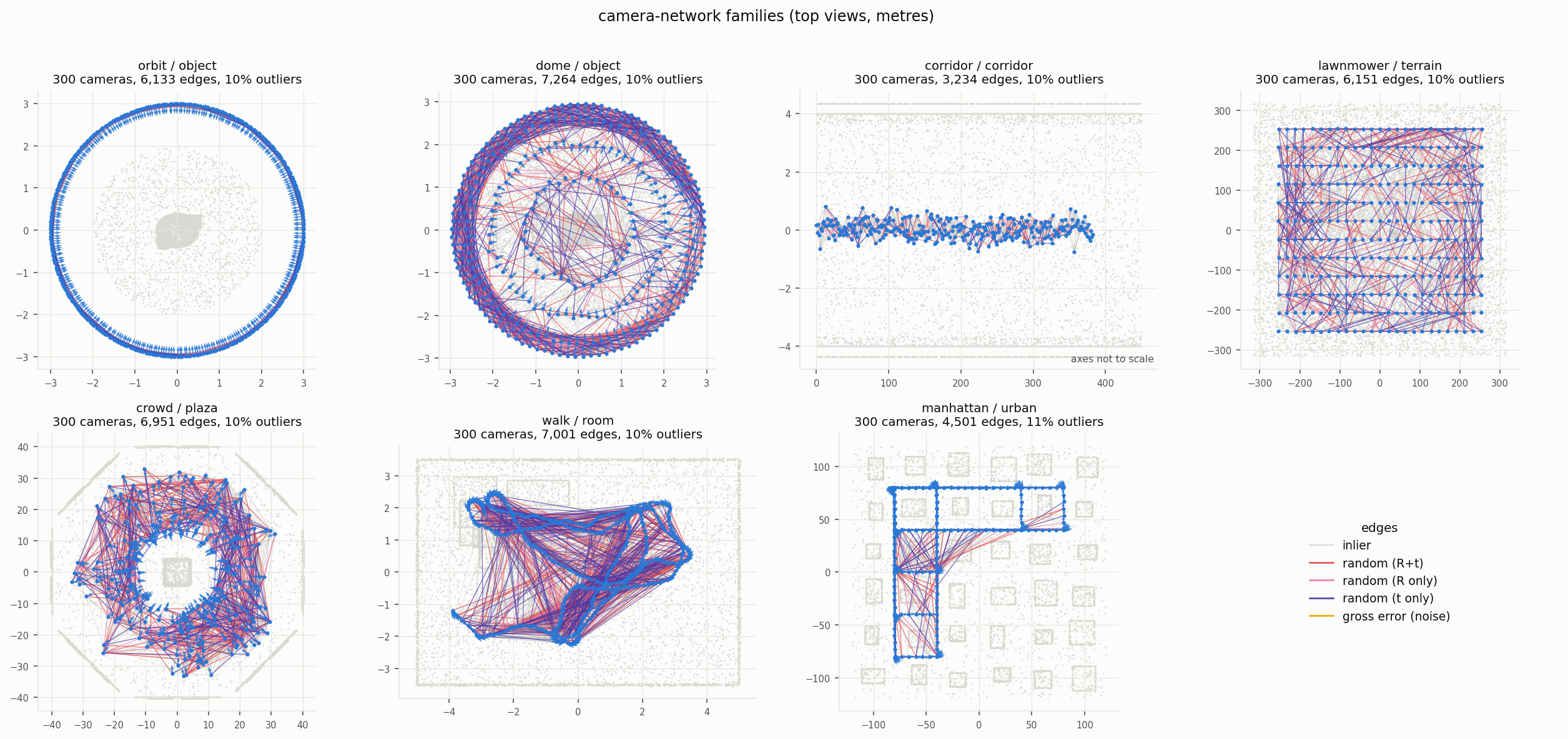
The seven camera-network families (top views of bench_topology graphs): cameras in blue, inlier edges in
grey, random outliers in red, pink and purple, gross errors of the noise model in yellow.
The package provides
- the generator: YAML configurations, parallel and resumable generation with a memory-aware scheduler;
- the
.npzgraph format with loaders, and g2o export and import; - baseline solvers for the four tasks, evaluation metrics and a benchmark runner with leaderboards;
- validation, statistics, figures, and the tools that prepare a dataset for the Hugging Face Hub.
Contents
- Installation
- Quick start
- The ViewGraphBench dataset
- How a graph is generated
- What a graph contains
- Generating datasets
- Benchmark
- Figures
- Command reference
- Parameter reference
- Examples
- Tests and reproducibility
- Troubleshooting
- Citation
- References
- License
1. Installation
pip install viewgraphforge
ViewGraphForge needs Python 3.10 or newer and depends on numpy, scipy, pandas, matplotlib and PyYAML. It is
pure Python and has been used on Linux and Windows. pip install "viewgraphforge[hub]" also installs
huggingface_hub 1.0 or newer, whose hf command downloads the dataset. For development:
git clone https://github.com/Ezharjan/ViewGraphForge.git
cd ViewGraphForge
pip install -e ".[dev]"
python -m pytest
2. Quick start
Generate a graph, run two baselines and save it:
import viewgraphforge as vgf
from viewgraphforge.benchmark import metrics, rotation_averaging, translation_averaging

g = vgf.generate_graph({"family": "crowd", "n_nodes": 200, "outlier_ratio": 0.2}, seed=1)
print(g.n_nodes, g.n_edges, g.is_outlier.mean())         # cameras, edges, fraction of outlier edges

R = rotation_averaging.l1_irls(g)                         # global rotations from the relative ones
print(metrics.rotation_metrics(R, g.R_wc)["rot_median_deg"])
C = translation_averaging.lud(g, R)                       # camera centres up to a similarity
print(metrics.position_metrics(C, g.centers)["pos_median_rel"])

vgf.save_graph(g, "crowd.npz")                            # also writes crowd.json with the metadata
vgf.write_g2o(g, "crowd.g2o")
On the command line, generate a small dataset (53 graphs in 11 splits) and run the tools on it:
vgf generate --config smoke --out data_smoke --workers 2
vgf validate --data data_smoke
vgf stats --data data_smoke
vgf benchmark --data data_smoke --workers 2
vgf visualize --data data_smoke
vgf --help lists all commands and vgf <command> --help explains the options of one.
3. The ViewGraphBench dataset
ViewGraphBench was generated with the full
configuration of this package (vgf config full prints it). It holds 45,495 graphs with about 15.2 million
cameras and 291 million relative-pose measurements in 16 splits:
| split | graphs | cameras requested | what varies |
|---|---|---|---|
train, val, test_wild |
40,000, 2,000, 2,000 | 30 to 800 | random draws of family, size, pixel noise, outlier ratio and type, retrieval depth, detection rate, noise model, heavy tails, scale noise and repeated structure |
test_wild_large |
200 | 800 to 5,000 | the same with larger graphs (analytic noise model only) |
bench_scale |
231 | 50 to 100,000 | number of cameras |
bench_noise |
147 | 300 | pixel noise, 0.25 to 16 px |
bench_outliers |
168 | 300 | fraction of random outliers, 0 to 0.6 |
bench_outlier_mode |
63 | 300 | what a random outlier replaces: rotation, direction or both |
bench_symmetry |
126 | 300 | confusability of repeated structure, 0 to 0.75 |
bench_density |
126 | 300 | retrieval depth, 3 to 80 views kept per camera |
bench_heavytail |
84 | 300 | Gaussian noise and Student-t noise with 5, 3 and 2 degrees of freedom |
bench_matches |
84 | 300 | minimum number of matches per edge, 10 to 80 |
bench_topology |
70 | 300 | camera-network family, 10 repetitions |
bench_twoview |
63 | 100, 300, 1,000 | number of cameras, with the simulated two-view estimator |
bench_twoview_symmetry |
28 | 300 | repeated structure, with the simulated two-view estimator |
bench_pgo |
105 | 500 | log-normal noise of the metric baseline lengths, 0.01 to 0.4 |
The benchmark splits vary one factor over the seven camera families (or over seven cases with repeated
structure), mostly with three repetitions. All levels of a factor use the same seed in a repetition, so the
scene, the cameras and the random numbers are the same up to the step where the factor acts. Download the
parts you need with the hf command (* also matches /):
pip install "viewgraphforge[hub]"
hf download ezharjan/ViewGraphBench --repo-type dataset --local-dir ViewGraphBench --include "splits/bench_*" --include "*.csv" --include "*.json" --include "manifest_sha256.txt"
import viewgraphforge as vgf

index = vgf.read_index("ViewGraphBench")                  # one row per graph: split, family, size, settings
rows = index[(index.split == "bench_outliers") & (index.outlier_ratio_target == 0.3)]
graphs = [vgf.load_graph(f"ViewGraphBench/{p}") for p in rows.npz_path]
The dataset card describes the files, the complete array layout, the statistics of every split and the baseline results.
4. How a graph is generated
Global SfM back ends are usually evaluated on view graphs of real photo collections such as those of 1DSfM [17], whose reference poses are themselves reconstructions, or on synthetic graphs with random topology, isotropic noise and uniformly random outliers. ViewGraphForge simulates the front end instead: edges, match counts and errors follow from a simulated scene and camera network, and the ground truth is exact. Each graph is generated from its own seed:
- Scene: a procedural point cloud with surface normals (object, facade, corridor, urban block, room, terrain or plaza) whose extent grows with the number of cameras for the corridor, urban, terrain and facade scenes. Scenes with repeated structure contain identical copies of a module: the sectors of a symmetric object, facade columns, corridor segments, twin buildings, the faces of a tower or a monument.
- Cameras: exactly
npinhole cameras (1600 x 1200 px) of one family:orbit(a ring around an object),dome(several rings on a hemisphere),corridor(forward motion along a street),lawnmower(an aerial survey),crowd(unordered photos of a landmark with varying focal lengths),walk(hand-held motion in a room) ormanhattan(a vehicle on a street grid, with loop closures). - Visibility: a point is observed when it is within the depth range, projects into the image, faces the camera, passes a z-buffer occlusion test and is detected; at most 3,000 points per image are kept.
- Edges: in graphs of up to 400 cameras every camera pair is a candidate; larger graphs take the nearest
neighbours in camera position and viewing direction, the three previous and next cameras in acquisition
order and, for repeated structure, random pairs of cameras that see copies of the same module. Match counts
are binomial in the number of co-visible points with a probability that falls with the angle between the
views and the scale change. Repeated structure adds competing hypotheses, and the reported relative pose is
drawn among those with enough matches, favouring the one with the most support. Each camera keeps its
retrieval_kcandidates with the most co-visible points and up tocand_sym_kidentical-looking views, a candidate becomes an edge when its reported pose has at leastmin_matchesmatches, and the largest connected component is kept. - Measurements: the reported relative pose with noise, from a closed-form model (
analytic) or from a simulated two-view estimator (twoview: the normalised 8-point algorithm [1] on noisy correspondences, Levenberg-Marquardt refinements of the Sampson error [10] from its solution and from the reported pose, of which the one with the lower error is kept, and covariances from the Fisher information). The analytic model is calibrated against the estimator: its errors scale with the pixel noise over the focal length and with 1/sqrt(matches), depend on the baseline-to-depth ratio and carry a log-normal factor per edge, with optional Student-t tails (analytic model only). - Outliers: a fraction of the edges, chosen with probability inversely proportional to their number of matches, receives random rotations and/or directions; the symmetry-induced outliers come from step 4. A metric translation is added for pose-graph optimisation, and every error is recorded.
5. What a graph contains
A graph is one compressed numpy archive (.npz) with n cameras and m edges, every camera pair stored once
with i < j. The main arrays:
| arrays | content |
|---|---|
node_q_wc, node_t_wc, node_center, node_K |
ground-truth world-to-camera rotation (quaternion) and translation, camera centre, intrinsics |
edge_i, edge_j |
the two cameras of an edge |
edge_q_meas, edge_tdir_meas, edge_t_meas |
measured relative rotation, unit translation direction and metric translation |
edge_q_true, edge_tdir_true, edge_t_true |
the same quantities from the ground-truth poses |
edge_sigma_rot, edge_sigma_dir, edge_sigma_trans |
noise levels reported for the measurement: standard deviations, or the Student-t scale with heavy tails |
edge_n_matches, edge_n_covis, edge_baseline, edge_median_depth, edge_view_angle_deg, edge_overlap_i, edge_overlap_j |
covariates of the edge |
edge_err_rot_deg, edge_err_dir_deg, edge_err_trans |
true errors of the measurement |
edge_outlier_type, edge_is_outlier, edge_symmetry_id |
outlier labels (table below) and the symmetry behind a symmetry-induced outlier |
points_*, obs_*, sym_* |
scene points, image observations of the points and the symmetry transforms behind the symmetry-induced outliers |
meta_json |
generation parameters, seed and statistics |
edge_outlier_type |
the measurement is |
|---|---|
0 none |
the true relative pose with noise (inlier) |
1 random_both |
a random rotation and a random direction |
2 random_rotation |
a random rotation with the noisy true direction |
3 random_translation |
a random direction with the noisy true rotation |
4 symmetry |
the relative pose, with noise, to a virtual camera: the true camera moved by a symmetry of the scene (for the translational symmetries of periodic facades and corridors, only the direction is wrong) |
5 gross_error |
not injected: a measurement of the noise model with an error above 10 deg in rotation or 20 deg in direction |
Conventions: metres, world frame with +z up, OpenCV camera frame (x right, y down, z forward), world-to-camera
poses x_cam = R_i X + t_i, relative poses R_ij = R_j R_i^T and t_ij = t_j - R_ij t_i, quaternions
(qx, qy, qz, qw) with qw >= 0. The .g2o files hold camera-to-world vertices (R_i^T, C_i) initialised
from a spanning tree of the measurements and EDGE_SE3:QUAT measurements Z_ij = (R_ij^T, -R_ij^T t_ij) with
their information matrices, whose rotation block refers to the rotation vector. GTSAM [15] reads them as they
are; for SE-Sync [16], remove the first line, a comment. g2o [14] reads them too, but its EdgeSE3 applies the
rotation block to the vector part of the quaternion, about half the rotation vector, which weights rotations four
times less (multiply the block by 4 to match). vgf.load_graph returns a PoseGraph with the arrays and
convenience properties (R_wc, centers, edges, R_meas, tdir_meas, t_meas, is_outlier, meta).
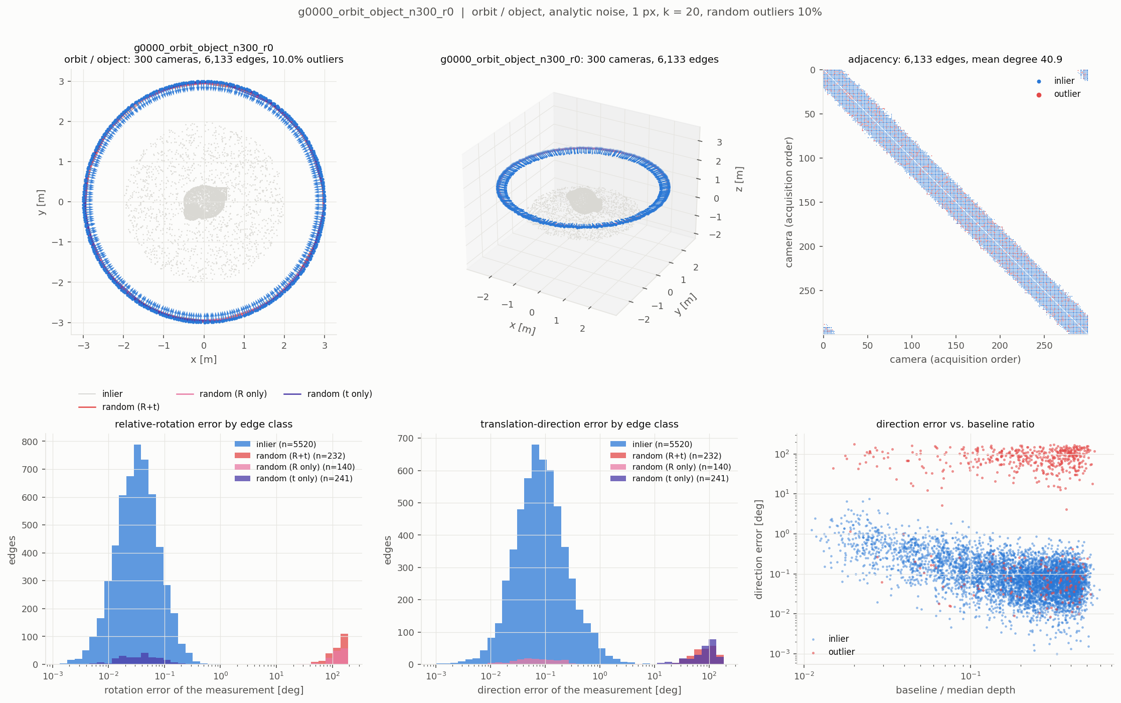
One graph in detail (vgf visualize): top and 3-D view, adjacency in acquisition order, the errors of each
edge class and the direction error against the baseline-to-depth ratio.
Repeated structure is what makes the symmetry-induced outliers (type 4) hard: every edge corrupted by the same symmetry agrees with the same moved camera, so the corrupted edges close their own cycles.
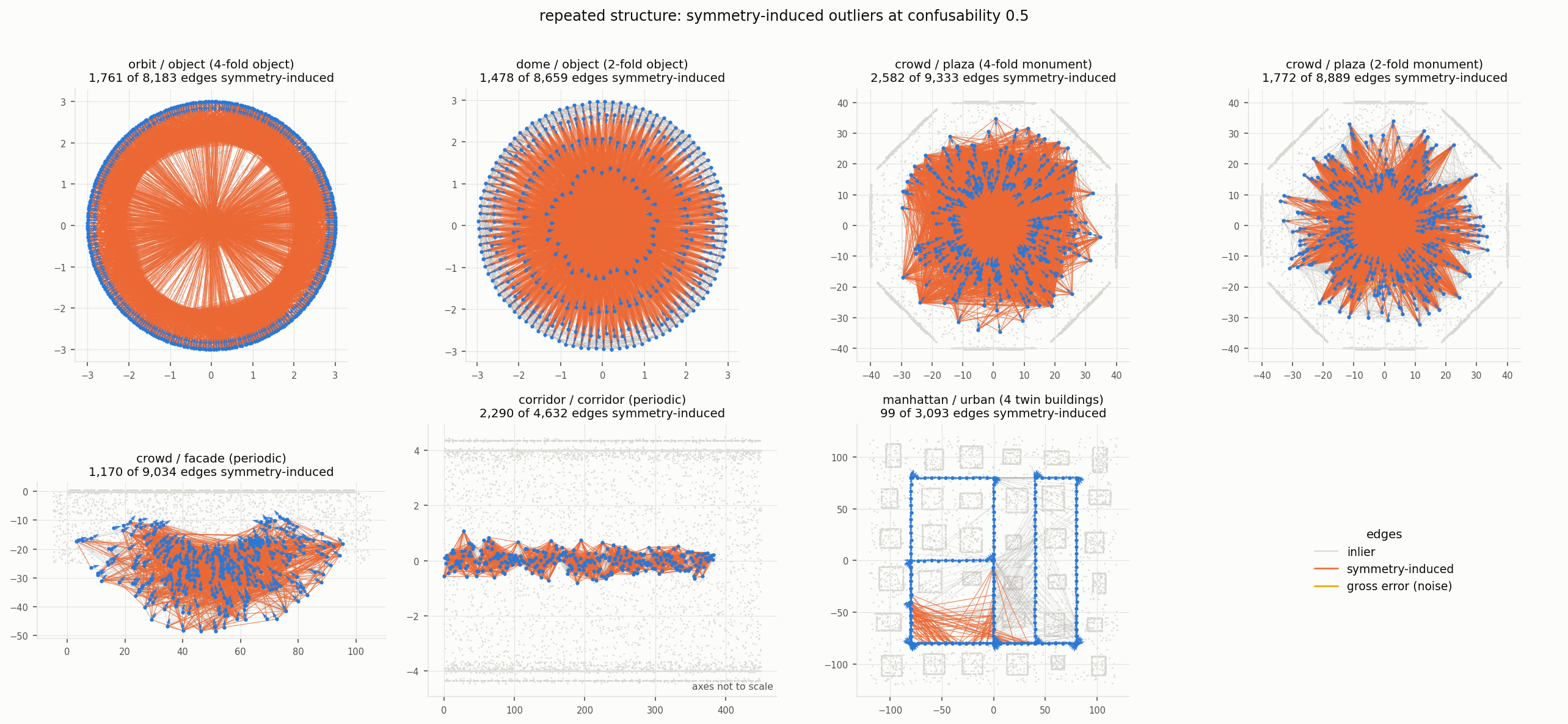
The seven cases with repeated structure of bench_symmetry at confusability 0.5; the orange edges are
symmetry-induced outliers. The twin buildings of the urban case produce few of them.
6. Generating datasets
A dataset is described by a YAML configuration. Two are shipped: smoke (53 graphs, for trying things out)
and full (the published dataset). vgf config lists them and vgf config full prints one.
vgf generate --config full --out data_full --workers 16
Each graph is written to <out>/splits/<split>/<graph_id>.npz together with a .json copy of its metadata and,
for graphs of up to 20,000 cameras (write_g2o_max_nodes), a .g2o file; splits of more than 3,000 graphs are
divided into folders of 1,000 graphs (splits/train/01000-01999/). At the end the command writes index.csv,
manifest_sha256.txt and dataset_info.json, and the log goes to <out>/logs/.
- Resuming. Running the same command again continues an interrupted run: finished graphs are kept, partial
files are removed and missing
.jsonor.g2ofiles are exported again from the.npz. All files are written atomically. A lock file keeps a second generator away from the same folder. - Memory. Graphs run in
--workersprocesses, largest first. A graph is started only when its estimated peak memory fits into the budget (--max-memory-gb, 70 % of the RAM by default) next to the memory the workers actually use, which the scheduler measures. The estimates are corrected by the peaks measured during the run, and a graph that still fails withMemoryErroris retried. Workers are replaced after 50 graphs or when they hold more than 1 GB, and the BLAS libraries run single-threaded inside them (through threadpoolctl when it is installed; without it, thread counts already set in the environment are kept). - Time and disk. The published dataset took about 13 hours with 16 workers on a laptop with 16 logical CPUs
and 32 GB of RAM, and takes 139 GB with the
.jsonand.g2ofiles. Most graphs of up to 1,000 cameras take seconds (thetwoviewgraphs up to a few minutes); the 100,000-camera graphs ofbench_scaletake from 3 minutes to 2.7 hours each and up to 4.3 GB of memory. The generator uses the CPU only. - Subsets and previews.
--splits train valgenerates some splits,--limit Nthe next N graphs, and--dry-run(with--listfor every graph) prints the plan without writing anything.
A configuration lists splits of three kinds. sweep varies one factor over a list of values, grid repeats
fixed settings and wild draws the settings at random:
dataset: {name: MyViewGraphs, version: "1.0.0", seed: 7}
generation: {workers: 8, write_g2o: true, write_json: true}
defaults: {store_points: true}                 # applied to every graph
splits:
  outliers:
    kind: sweep
    factor: outlier_ratio
    values: [0.0, 0.2, 0.4]
    families: all                              # or a list, e.g. [orbit, crowd]
    seeds: 5
    params: {n_nodes: 500}
  corridors:
    kind: grid
    families: [corridor]
    seeds: 20
    params: {n_nodes: 1000, noise_model: twoview}
  training:
    kind: wild
    count: 5000
    sampler: {n_nodes: {min: 50, max: 2000, log: true, int: true}}
Every graph parameter of section 10 can appear in defaults, params or as the
factor of a sweep. In a wild split the values drawn by the sampler take precedence over defaults and
params; their ranges are set in sampler (the keys of DEFAULT_WILD_SAMPLER in viewgraphforge/splits.py).
vgf config smoke > my.yaml writes a complete example to start from.
7. Benchmark
vgf benchmark --data ViewGraphBench --splits "bench_*" "test_*" --workers 16
runs the baselines on the graphs of the selected splits and writes benchmarks/results.csv (one row per graph
and method), leaderboard.csv and leaderboard.md (means per split and method), sweeps.csv (metrics against
the swept factor) and run.json (settings and software versions). Results are cached, so an interrupted run
continues where it stopped. By default graphs with more than 3,000 cameras are skipped (--max-nodes), and
pose-graph optimisation runs on graphs of up to 1,500 cameras (--max-nodes-pgo).
| task | baselines | metrics |
|---|---|---|
| rotation averaging | spanning tree; chordal L2 [2]; chordal L2 with Cauchy IRLS; L1 averaging followed by IRLS [4, 5, 6], with and without information weights | rotation errors after robust alignment of the global rotation: median, mean, RMS, 90th percentile, fraction below 1, 3, 5 and 10 deg |
| translation averaging | linear cross-product method [3]; least unsquared deviations, LUD [7]; each with ground-truth and with L1-IRLS rotations | position errors after a similarity alignment [11], absolute and relative to the extent of the cameras |
| pose-graph optimisation | spanning-tree initialisation; Levenberg-Marquardt with exact SE(3) Jacobians [12, 13] and L2, Huber and Cauchy losses; Cauchy from a rotation-averaging initialisation [9] | position and rotation errors after a rigid alignment, iterations |
| outlier detection | triangle cycle consistency [8]; rotation residuals after L1-IRLS; direction residuals after LUD | precision, recall, F1 and average precision against the edges with a rotation error above 5 deg (direction error above 10 deg); graphs without such edges are left out of the means |
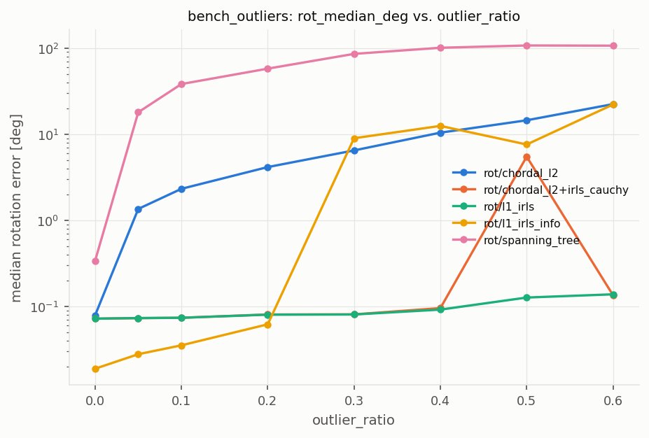
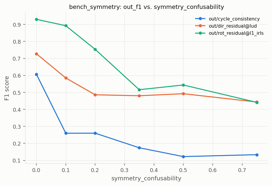
Left: median rotation error against the fraction of random outliers (bench_outliers). Right: F1 score of
outlier detection against the confusability of repeated structure (bench_symmetry); cycle consistency misses
almost all symmetry-induced outliers. Each point is the mean over the 21 graphs of one level (for F1, over those
with labelled outliers).
A method of your own is a function of the graph; registered in the method table, it is evaluated with the same
protocol by the serial runner (the worker processes of vgf benchmark know only the built-in methods):
from viewgraphforge.benchmark import rotation_averaging, runner

rotation_averaging.ROTATION_METHODS["rot/my_method"] = my_solver    # graph -> (n,3,3) world-to-camera rotations
results = runner.run_dataset("ViewGraphBench", splits=["bench_outliers"], tasks=["rotation"])
examples/09_benchmark_and_leaderboard.py does this and builds the leaderboard and the sweep plots.
8. Figures
vgf visualize --data <folder> renders into <folder>/figures/: the family and symmetry overviews above,
per-graph overviews, a gallery of every split, the dataset summary, the sweep curves and leaderboard bars of the
benchmark, and solver results on a few graphs such as the one below. The plotting functions are available in
viewgraphforge.viz (see examples/10_visualize_dataset.py).
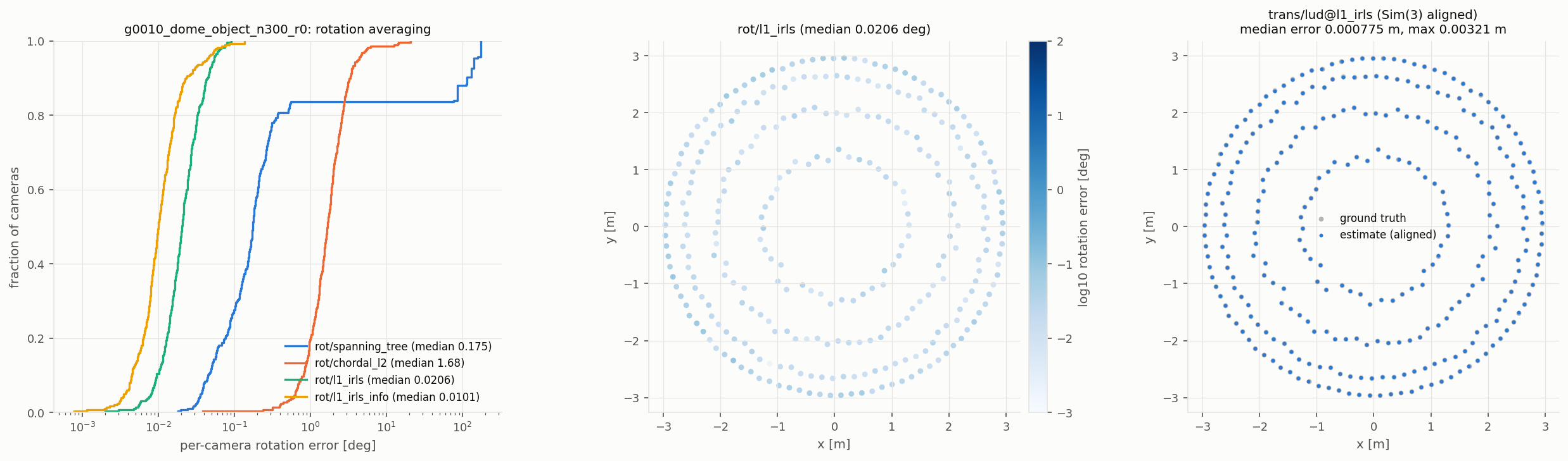
A dome graph with 300 cameras and 10 % outliers: per-camera rotation errors of four rotation-averaging methods, the errors of L1-IRLS on the cameras, and the camera centres from LUD after a similarity alignment.
9. Command reference
| command | purpose |
|---|---|
vgf generate --config <name or file> --out <folder> |
generate a dataset; parallel, resumable, memory-aware |
vgf validate --data <folder> |
check every graph, its .g2o file, index.csv and the SHA-256 manifest |
vgf stats --data <folder> |
statistics per graph and per split in stats/ |
vgf benchmark --data <folder> |
run the baselines and write the leaderboards in benchmarks/ |
vgf visualize --data <folder> |
render the figures in figures/ |
vgf export --data <folder> --out <folder> |
assemble the files published on the Hugging Face Hub (hard links, sub-folders for large splits) |
vgf card --data <folder> |
write the dataset card (README.md) from the files of a folder |
vgf config [name] |
list the shipped configurations or print one |
vgf calibrate |
fit the analytic noise model to the simulated two-view estimator |
vgf clean |
remove caches, build files and the leftovers of interrupted runs; --data <folder> --wipe deletes a dataset |
validate, stats and benchmark accept --workers N. The --splits option of generate, validate,
benchmark and visualize takes split names or shell-style patterns such as "bench_*", as does --g2o of
export; stats reads every split. python -m viewgraphforge is the same as vgf.
10. Parameter reference
Graph parameters with their defaults (viewgraphforge/config.py):
| parameters | defaults | meaning |
|---|---|---|
family, scene |
orbit, family default |
camera family (orbit, dome, corridor, lawnmower, crowd, walk, manhattan) and scene (object, facade, corridor, urban, room, terrain, plaza) |
n_nodes |
200 | number of cameras; the largest connected component of the view graph is kept |
n_points, scene_params |
scale-aware | scene points and options of the scene builder, e.g. {symmetry_fold: 4}, {periodic: true}, {tower_fold: 4}, {twin_buildings: 4}, {monument_fold: 2} |
camera_params, image_size, hfov_deg |
family defaults, 1600 x 1200 | options of the camera family and intrinsics |
detection_prob, max_depth_factor, max_depth_abs, max_incidence_deg, zbuffer_tol, max_visible_per_camera |
0.8, 6, 400 m, 80 deg, 0.08, 3000 | visibility model |
retrieval_k, min_matches, p_match_max, theta0_deg, s0, hypothesis_sharpness |
20, 20, 0.7, 40 deg, 0.7, 4 | retrieval depth, minimum matches of an edge, match probability model and selection among competing hypotheses |
symmetry_confusability, cand_sym_k |
0, 4 | factor on the match probability of correspondences between two copies of repeated structure (0: never confused); retrieval budget per camera for identical-looking views |
noise_model, pixel_noise, heavy_tail_df, scale_noise |
analytic, 1 px, 0 (Gaussian), 0.05 |
measurement noise; twoview runs the simulated two-view estimator |
outlier_ratio, outlier_mode, outlier_weighting |
0.1, mixed, inverse_matches |
random outliers: fraction, type (rotation, translation, both, or mixed: both, translation and rotation with probabilities 0.4, 0.4 and 0.2) and choice of the edges |
gross_rot_deg, gross_dir_deg |
10 deg, 20 deg | thresholds of the gross_error label |
store_points, max_points_stored, store_observations, store_observations_max_nodes, max_observations_per_camera |
true, 20000, true, 2000, 300 | stored scene points and image observations |
The constants of the analytic noise model (viewgraphforge/noise.py) were fitted with
vgf calibrate --n-nodes 100 --seeds 3 on a development version of the generator (28,715 inlier edges;
viewgraphforge/configs/noise_calibration.json holds the fit). The released version gives similar but not
identical constants (about 29,800 edges, a_rot 35.4 instead of 36.7); the shipped constants are kept so that
ViewGraphBench can be regenerated.
11. Examples
The examples run on the smoke dataset
(vgf generate --config smoke --out data_smoke --workers 2) or on a downloaded copy of ViewGraphBench:
| example | shows |
|---|---|
01_load_and_inspect.py |
the arrays of a graph and a check of the pose, relative-pose and epipolar conventions |
02_rotation_averaging.py |
rotation averaging by spanning tree, chordal L2, chordal L2 with Huber IRLS and L1-IRLS, and the error distributions |
03_translation_averaging.py |
world-frame baseline directions, the linear method and LUD with true and estimated rotations |
04_pose_graph_optimization_g2o.py |
robust SE(3) pose-graph optimisation from a .g2o file, with an optional GTSAM cross-check |
05_outlier_filtering.py |
cycle-consistency and residual filters, and why symmetry-induced outliers defeat cycle consistency |
06_learning_edge_classifier.py |
per-edge features, conversion to PyTorch Geometric and a learned outlier classifier on the wild splits |
07_point_based_global_positioning.py |
camera positions from the image observations, the idea behind the global positioning of GLOMAP [18], where camera-only translation averaging fails |
08_custom_generation.py |
generating graphs from Python with repeated structure, two-view noise and heavy tails |
09_benchmark_and_leaderboard.py |
the benchmark runner with a method of your own, a leaderboard and a sweep plot |
10_visualize_dataset.py |
the plotting functions of viewgraphforge.viz |
12. Tests and reproducibility
python -m pytest runs the test suite: the exponential and logarithm maps of SO(3) and SE(3), the SE(3)
Jacobians against finite differences, the pose, quaternion and projection conventions, the invariants of
generated graphs of every family, the exact consistency of noise-free graphs, the virtual-camera relation of
symmetry-induced outliers, the two-view estimator, the npz and g2o round trips, determinism, the solvers and
metrics on clean and corrupted graphs, and the commands (parallel generation, resume, lock, scheduler,
validation, export, dataset card, clean).
Every graph has a 32-bit seed, SeedSequence(dataset_seed, spawn_key=key).generate_state(1, uint32)[0] with
key = (crc32(s), k) for graph k of a wild split s and key = (crc32(s), c, r) for case c and
repetition r of a sweep or grid split (column seed of index.csv), whatever the number of workers and
the order of execution. The graph is generated with numpy.random.default_rng(seed); the settings of a wild
graph are drawn before, with default_rng(SeedSequence(seed, spawn_key=(7,))). On the same platform and library
versions a configuration therefore reproduces every array of every graph exactly; only the generation times
stored in each file differ, so the file hashes of two runs differ. Elsewhere the last bits of
floating-point results can differ, which can change a visibility or matching decision and then the rest of that
graph. Regenerated on Linux with numpy 2.5.3 and scipy 1.18.1, 61 benchmark graphs of the published copy (made on
Windows) kept their edges, match counts and labels, while 3 of 7 training graphs (two with the twoview
estimator, one with more than 400 cameras) did not; with numpy 2.4.4 and scipy 1.17.1, 26 of the 61 benchmark
graphs differed as well. Datasets from different machines are therefore compared with vgf validate and
vgf stats rather than by file hash.
13. Troubleshooting
MemoryErrorin the log. The machine ran out of memory, often because other programs use a large share of it. Lower the budget (--max-memory-gb) or the number of workers and run the same command again; failed graphs are generated on the next run.- Generation is slow and the CPU is mostly idle. The machine is swapping. Check the memory figures in the log
lines and lower
--max-memory-gb,--workersor--recycle-gb. High CPU use with slow progress points toOMP_NUM_THREADSorMKL_NUM_THREADSset above 1 in the environment, which the workers keep when threadpoolctl is not installed. another vgf generate (pid ...) is writing to .... A secondvgf generateon the same folder was refused. A lock left by a crashed run is removed automatically;--forceoverrides the check.- A graph has fewer cameras than its id says. Only the largest connected component is kept; the id records
the requested number,
index.csvand the metadata the actual one. - Rows of two tables do not match. A graph id is unique within its split but can occur in several splits, so
tables are joined on (
split,graph_id). - Translation averaging fails on
corridorandmanhattangraphs. The directions between cameras on a straight path do not determine their spacing. The image observations do (examples/07_point_based_global_positioning.py).
14. Citation
If you use the dataset or the software, please cite the dataset:
@misc{viewgraphbench2026,
  title        = {ViewGraphBench: Physically-Grounded Synthetic View Graphs for Global Structure-from-Motion Calibration},
  author       = {Aiersilan, Aizierjiang},
  year         = {2026},
  note         = {Dataset version 1.0.0, generated with ViewGraphForge},
  howpublished = {Hugging Face Hub},
  url          = {https://huggingface.co/datasets/ezharjan/ViewGraphBench}
}
To refer to the software itself:
@software{viewgraphforge2026,
  title        = {ViewGraphForge},
  author       = {Aiersilan, Aizierjiang},
  year         = {2026},
  url          = {https://github.com/Ezharjan/ViewGraphForge}
}
CITATION.cff holds the same information in
the Citation File Format.
15. References
- R. Hartley. In defense of the eight-point algorithm. IEEE TPAMI 19(6):580-593, 1997.
- D. Martinec and T. Pajdla. Robust rotation and translation estimation in multiview reconstruction. CVPR 2007.
- V. M. Govindu. Combining two-view constraints for motion estimation. CVPR 2001.
- V. M. Govindu. Lie-algebraic averaging for globally consistent motion estimation. CVPR 2004.
- A. Chatterjee and V. M. Govindu. Efficient and robust large-scale rotation averaging. ICCV 2013.
- A. Chatterjee and V. M. Govindu. Robust relative rotation averaging. IEEE TPAMI 40(4):958-972, 2018.
- O. Özyeşil and A. Singer. Robust camera location estimation by convex programming. CVPR 2015.
- C. Zach, M. Klopschitz and M. Pollefeys. Disambiguating visual relations using loop constraints. CVPR 2010.
- L. Carlone, R. Tron, K. Daniilidis and F. Dellaert. Initialization techniques for 3D SLAM: a survey on rotation estimation and its use in pose graph optimization. ICRA 2015.
- P. D. Sampson. Fitting conic sections to "very scattered" data: an iterative refinement of the Bookstein algorithm. Computer Graphics and Image Processing 18(1):97-108, 1982.
- S. Umeyama. Least-squares estimation of transformation parameters between two point patterns. IEEE TPAMI 13(4):376-380, 1991.
- T. D. Barfoot. State Estimation for Robotics. Cambridge University Press, 2017.
- J. Solà, J. Deray and D. Atchuthan. A micro Lie theory for state estimation in robotics. arXiv:1812.01537, 2018.
- R. Kümmerle, G. Grisetti, H. Strasdat, K. Konolige and W. Burgard. g2o: a general framework for graph optimization. ICRA 2011.
- F. Dellaert. Factor graphs and GTSAM: a hands-on introduction. Technical report GT-RIM-CP&R-2012-002, Georgia Institute of Technology, 2012.
- D. M. Rosen, L. Carlone, A. S. Bandeira and J. J. Leonard. SE-Sync: a certifiably correct algorithm for synchronization over the special Euclidean group. International Journal of Robotics Research 38(2-3):95-125, 2019.
- K. Wilson and N. Snavely. Robust global translations with 1DSfM. ECCV 2014.
- L. Pan, D. Baráth, M. Pollefeys and J. L. Schönberger. Global structure-from-motion revisited. ECCV 2024.
16. License
MIT License, Copyright (c) 2026 Aizierjiang Aiersilan. See LICENSE.
1 maintainer

Release files for viewgraphforge 1.0.0
For a detailed explanation of source distributions (sdists) and built distributions (wheels), please see the package formats documentation.
Source distribution (sdist)
| File | Size | Uploaded | |
|---|---|---|---|
| viewgraphforge-1.0.0.tar.gz | 228.6 kB | Details |
Built distribution (wheel)
| File | Interpreter | ABI | Platform | Reset |
|---|---|---|---|---|
| viewgraphforge-1.0.0-py3-none-any.whl | Python 3 | none | any | Details |
Total release size: 427.3 kB
Release files / viewgraphforge-1.0.0.tar.gz
| Download URL | viewgraphforge-1.0.0.tar.gz |
|---|---|
| Size | 228.6 kB |
| Tags | Source |
|
SHA-256 checksum How to use checksums |
55321c5043d7c4e44d1b96789b8d853ffacef5aea8762a088790608a61843113
|
|
BLAKE2b-256 checksum How to use checksums |
6e09f1af07a3ce99c14af5d1ab18f72fa8aa7f9bc34b1f44b67c717a7aa3370e
|
| Upload date | |
|
Uploaded using Trusted Publishing? What is trusted publishing? |
No |
| Uploaded via |
twine/7.0.0 CPython/3.12.12
|
Release files / viewgraphforge-1.0.0-py3-none-any.whl
| Download URL | viewgraphforge-1.0.0-py3-none-any.whl |
|---|---|
| Size | 198.8 kB |
| Tags | Python 3 |
|
SHA-256 checksum How to use checksums |
0d73307021c8dd0b4a7f83b787b34bcf1eae85cff889277e82c6796ba41bd1c9
|
|
BLAKE2b-256 checksum How to use checksums |
035c1c219d1c0b49f8a5d431509b97e5db1b87a2b74a9c7eb307cb1450e1bd35
|
| Upload date | |
|
Uploaded using Trusted Publishing? What is trusted publishing? |
No |
| Uploaded via |
twine/7.0.0 CPython/3.12.12
|













