
This release is a pre-release and may not be stable for production use.






Useful tools for data visualisation, e.g. 2D-profiles, comparison of measurements, or tables.
[!WARNING] This package is still under development. The features work, but the API might change in the future.
Developed and maintained by Philipp Meder.
- Source code: https://github.com/philippmeder/visdata
- Report bugs: https://github.com/philippmeder/visdata/issues
Quick Start
Install this package:
pip install visdata
You can get the newest stable version with:
pip install git+https://github.com/philippmeder/visdata
License
Distributed under the BSD 3-Clause License.
Features
This README covers the following:
- Profile2d Plot for 2D-histograms
- Visual Comparison of Measurements
- Table Output for Terminal, CSV, and LaTeX
- Additional Features
Check out the examples!
Profile2d Plot for 2D-histograms
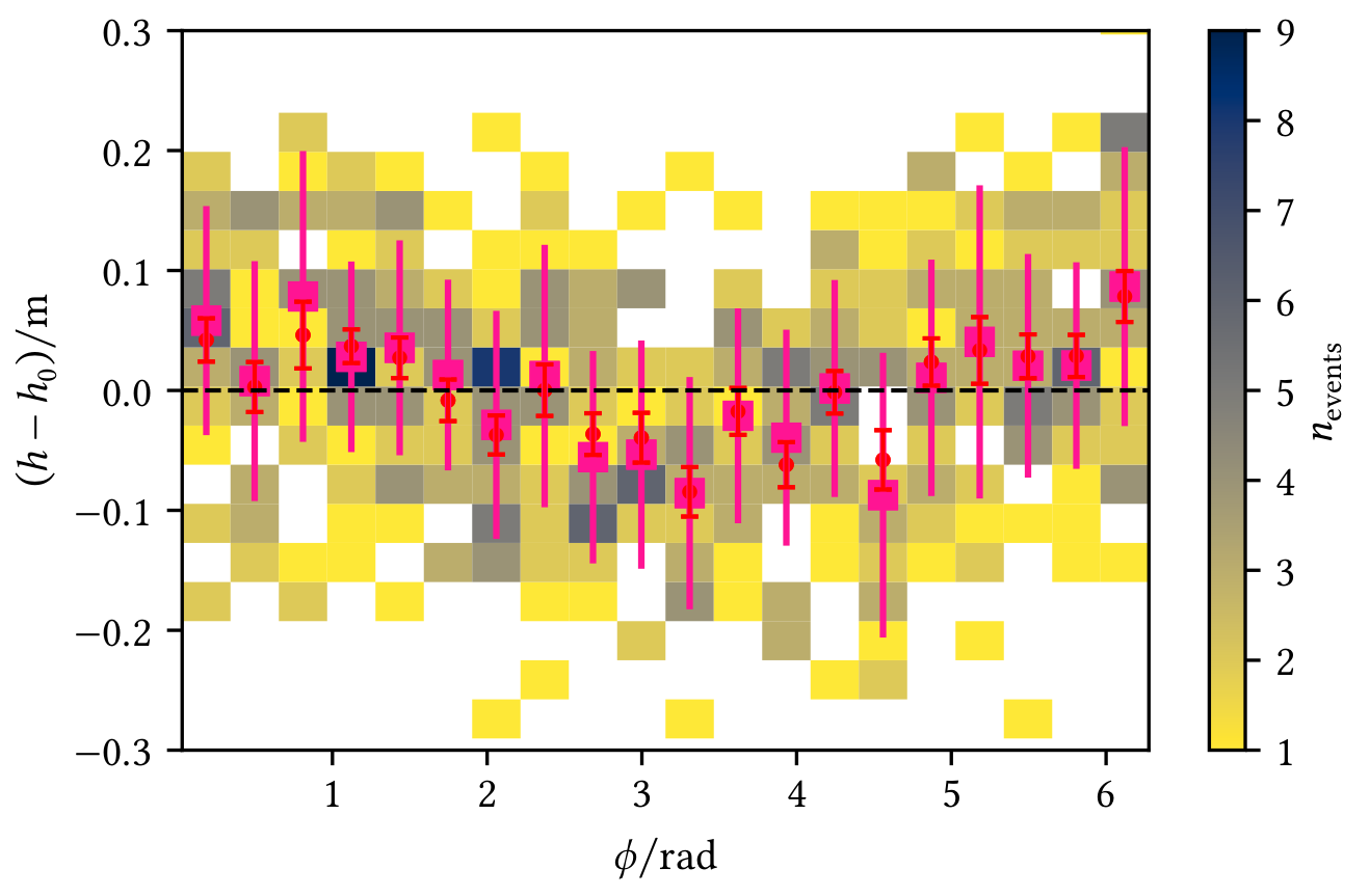
Profiles allow a visual interpretation of the data, e.g. in the following figures where red markers represent the mean with the standard error on the mean and pink markers represent the median of the y-data in each x-bin:
| Profile shows an angle-dependent deviation from the zero line | Profile shows deviations from the model |
|---|---|
 |
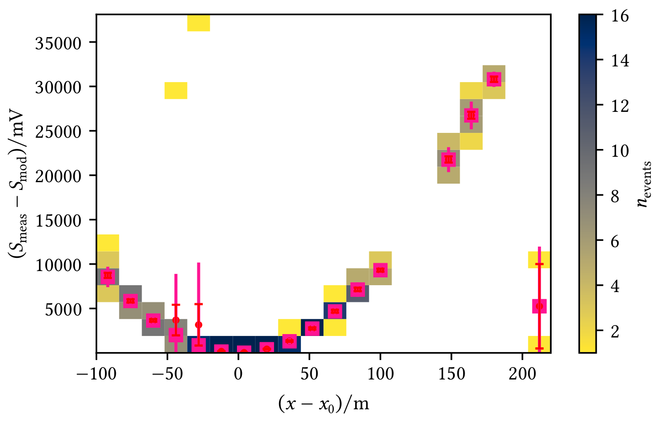 |
Create a Profile2d object with your data and directly add the profile to a plot (you may adjust what and how to plot, see Histogramd2d example) or get the profile data and do the plotting yourself.
from matplotlib import pyplot as plt
from visdata import Profile2d, plot_profile2d

# Example data
x, y = ...

# Create normal 2D-histogram
fig, ax = plt.subplots()
hist, xedges, yedges, image = ax.hist2d(x, y, bins=10)

# Create profile and add it to the axis (using default config)
profile = Profile2d(x, y, bins=10)
plot_profile2d(ax, profile)
You can also use a Histogram2d object which gives you the ability to directly draw a profile.
In addition, it allows to plot 1D-histograms of the x/y data on the margins, which looks like this:
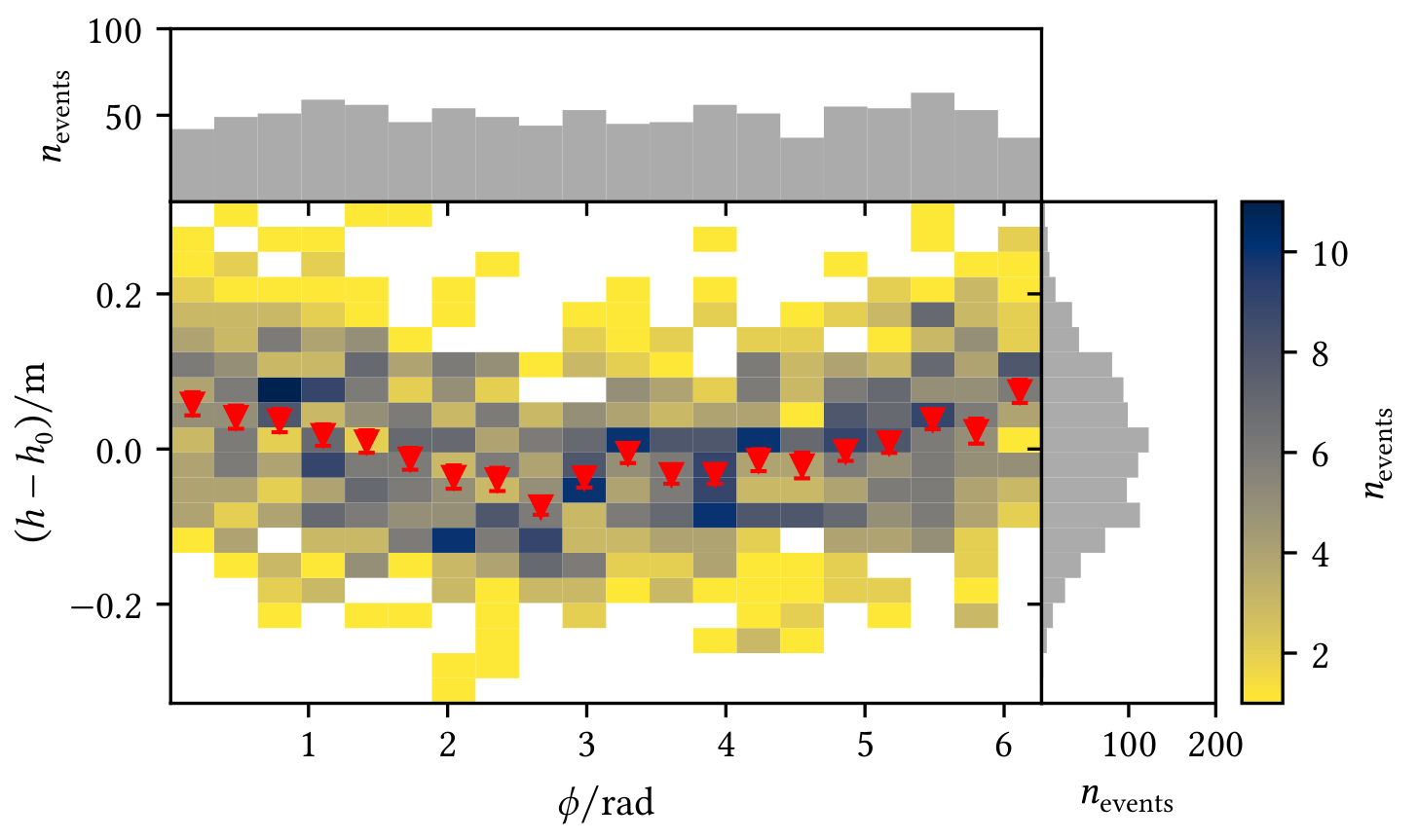
You can configure the marginal plots and the profile, see the following example:
from visdata import Histogram2d, Profile2dMeanPlotter, plot_profile2d

hist = Histogram2d(x, y, bins=bins)
# Configure the marginal histograms if wanted, e.g. the color
# Keywords are passed to 'ax.hist'
hist.configure_marginal(color="C2")
# Configure the profile with a set of configs, e.g. only plot the mean but change the marker
hist.profile_plotters = [
    # Keywords are passed to 'ax.errorbar'
    Profile2dMeanPlotter(marker="v")
    # You could add another config here, e.g. to plot the median
]
# Plot hist2d with colorbar + 1D-histograms and profile
hist_result = hist.plot(marginal=True, profile=True)
Visual Comparison of Measurements Including Uncertainties
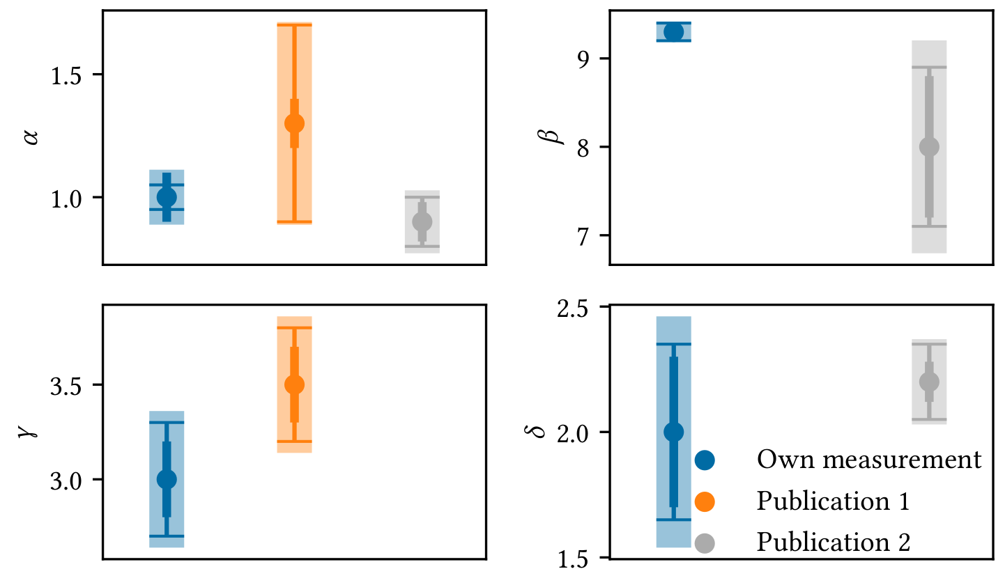
Sometimes it is easier to understand if different measurements are compatible with each other by looking at a visualisation, e.g. you want to compare your own measurements of some parameters with the measurements presented in other publications with respect to the uncertainties. The example shows
- statistical uncertainties as medium thick errorbars,
- systematic uncertainties as thin errorbars with caps,
- quadratic combination of both as thick errobars with transparency (for visual guidance only, this value is meaningless).
You can of course configure what and how to plot. In this example, Publication 1 did not provide any values for $\beta$ and $\delta$ while Publication 2 did not provide a value for $\gamma$.
from visdata import (
    Measurement, MeasurementResult, CompareMeasurementsPlot
)

# Example measurements for multiple parameters
measurement_1 = Measurement(
    "Measurement name",
    {
        "par 1 name": MeasurementResult(
            1, statistical=0.1, systematic=0.05
        ),
        ...
    }
)
measurement_2 = ...

# Create plot object and do the plotting
comp_plot = CompareMeasurementsPlot(measurment_1, measurement_2)
fig, axs, handles, labels = comp_plot.plot()

# At this point you can configure fig and axs the usual way or include a legend with handles and labels
...
Formatted Table Output for Terminal, CSV, and LaTeX
Create a Table object from a 2D-array and get the wanted output, either as a nice terminal output, a CSV table, or a LaTeX table ready for your document.
You can name the columns and rows independently and add a caption if you want. Furthermore, you can specify a formatter for the data.
from visdata import Table

# Setup data and example formatter
data, description, column_labels, row_labels = ...
formatter = "5.2f"

# Create table object
table = Table(
    data,
    description=description,
    column_labels=column_labels,
    row_labels=row_labels
)
# Print the terminal representation as well as CSV and LaTeX
print(table)
print(table.csv(formatter=formatter))
print(table.latex(formatter=formatter))
The LaTeX output returns a scientific table. The terminal representation mimics this, e.g.
            Table: Some important values
────────────────────────────────────────────────────
              a0            a1            a2
────────────────────────────────────────────────────
A0              0.00e+00      1.00e+00      2.00e+00
A1              3.00e+00      4.00e+00      5.00e+00
────────────────────────────────────────────────────
Additional Features
- Decorators for code development, e.g. timer for function execution
- Intervals
- Functions like secans or cos called with angle in degrees
- Regular polygons for plotting and calculation of their most important properties
- Some utilities for matplotlib output
Requirements and Dependencies
Following requirements must be satisfied:
Python 3.10+(developed withPython 3.13, tested withPython 3.10+, lower version are not working due to the use ofmatch ... caseandUnion)numpy 2+matplotlib 3.8+
1 maintainer

Metadata
1 maintainer
Release files for visdata 0.2.0.dev1
For a detailed explanation of source distributions (sdists) and built distributions (wheels), please see the package formats documentation.
Source distribution (sdist)
| File | Size | Uploaded | |
|---|---|---|---|
| visdata-0.2.0.dev1.tar.gz | 26.1 kB | Details |
Built distribution (wheel)
| File | Interpreter | ABI | Platform | Reset |
|---|---|---|---|---|
| visdata-0.2.0.dev1-py3-none-any.whl | Python 3 | none | any | Details |
Total release size: 51.5 kB
Release files / visdata-0.2.0.dev1.tar.gz
| Download URL | visdata-0.2.0.dev1.tar.gz |
|---|---|
| Size | 26.1 kB |
| Tags | Source |
|
SHA-256 checksum How to use checksums |
d21cf810a546daed52de98fc018f4c7fdd5086ebe6cd71ac553ff564b8f7db42
|
|
BLAKE2b-256 checksum How to use checksums |
a82da3a11f71dfe0496889ee13b846dd77e52c3510f18b93e5e4d8d9e97814dd
|
| Upload date | |
|
Uploaded using Trusted Publishing? What is trusted publishing? |
Yes |
| Uploaded via |
twine/6.1.0 CPython/3.12.9
|
Provenance
Provenance describes where a file came from. On PyPI, provenance is shared via attestations, which provide a verifiable record of the build or publishing details. View details, limitations and caveats.


PyPI Publish Attestation
PyPI verified that this artifact, at this checksum, originated from the publisher listed below.
Signed by GitHub Actions, verified by PyPI on Aug 4, 2025.
Transparency logRelease files / visdata-0.2.0.dev1-py3-none-any.whl
| Download URL | visdata-0.2.0.dev1-py3-none-any.whl |
|---|---|
| Size | 25.4 kB |
| Tags | Python 3 |
|
SHA-256 checksum How to use checksums |
7db3e26ee2653f9ec3d3ba45af9bf30553d56aa15493ea31226a8e47c07ac478
|
|
BLAKE2b-256 checksum How to use checksums |
c5039c331264eafa75cfe170c349a1536077dd0515fdba928b91770cd21cb20d
|
| Upload date | |
|
Uploaded using Trusted Publishing? What is trusted publishing? |
Yes |
| Uploaded via |
twine/6.1.0 CPython/3.12.9
|
Provenance
Provenance describes where a file came from. On PyPI, provenance is shared via attestations, which provide a verifiable record of the build or publishing details. View details, limitations and caveats.
PyPI Publish Attestation
PyPI verified that this artifact, at this checksum, originated from the publisher listed below.
Signed by GitHub Actions, verified by PyPI on Aug 4, 2025.
Transparency log












