
A PSO library with a focus on visualization.

Project description
Visual Swarm
A modern, visualization-first Particle Swarm Optimization (PSO) library for Python.
Visual Swarm makes it easy to not only run PSO but to see it in action. It's designed for researchers, students, and developers who want to gain an intuitive understanding of how swarms explore a search space.
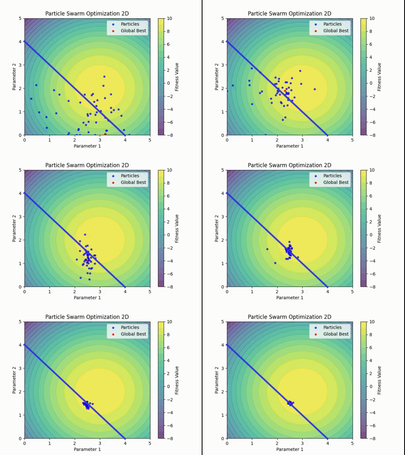
! The constraint line in blue has been added by editing the generated videp and is not available through code. The constraints may take form that I cannot account for when coding the visualization function
Table of Contents
Key Features
- Built-in Animations: Generate 1D, 2D, and 3D animations of the optimization process with a single line of code.
- Save to Video: Save your animations directly to
.mp4files for presentations or reports. - Modern API: A clean, object-oriented interface that's easy to extend.
- Flexible Topologies: Switch between global best (gbest) and local best (lbest) PSO with a simple boolean flag.
- Constraint Handling: Easily define constraints and penalties for complex optimization problems.
Installation
To save animations, you will need FFmpeg installed on your system.
# On macOS (using Homebrew):
brew install ffmpeg

# On Debian/Ubuntu:
sudo apt-get install ffmpeg

# On Windows (using Chocolatey):
choco install ffmpeg
Once FFmpeg is installed, you can install Visual Swarm and its dependencies:
There are two ways to install Visual Swarm: 1. For Development :
# Clone the repository and install in editable mode for development
git clone https://github.com/AnshulPatil29/visual-swarm.git
cd visual-swarm
pip install -e .
2. For General Use :
pip install visual-swarm
Quick Start: 2D Optimization
Here's how easy it is to find the peak of a 2D function and watch the swarm converge.
import numpy as np
import matplotlib.pyplot as plt
from visual_swarm import ParticleSwarm

# 1. Define a fitness function to maximize
def peak_function(x, y):
    return -((x - 3)**2 + (y - 2)**2) + 10

# 2. Define the search space bounds: [[x_min, x_max], [y_min, y_max]]
bounds = np.array([[0.0, 5.0], [0.0, 5.0]])

# 3. Initialize the optimizer
pso = ParticleSwarm(
    num_particles=50,
    fitness_function=peak_function,
    bounds=bounds
)

# 4. Create the animation! This also runs the optimization.
# show_grid=True helps visualize the fitness landscape.
ani = pso.create_animation(iterations=100, show_grid=True)

# 5. Show the final results and the animation plot
print(f"Best solution found: {pso.global_best_particle}")
print(f"Best fitness: {pso.global_best_fitness:.4f}")
plt.show()
Advanced Usage
Saving an Animation
To save the animation to a file instead of viewing it interactively, use the save and save_path arguments.
# Creates a file named '2d_peak_optimization.mp4' in the current directory
pso.create_animation(
    iterations=100,
    show_grid=True,
    save=True,
    save_path='2d_peak_optimization.mp4'
)
Local Best PSO (lbest)
To help avoid premature convergence on complex problems, you can use the local best topology. Each particle is influenced by the best particle in its immediate neighborhood, not the entire swarm.
pso_local = ParticleSwarm(
    num_particles=50,
    fitness_function=peak_function,
    bounds=bounds,
    is_global=False,          # Set to False for local best
    neighborhood_size=5       # Define how many neighbors to consider
)
AI Assistance
To enhance productivity and ensure high-quality documentation, this project utilized AI assistance (via Google's Gemini) for the following specific tasks:
- Generating initial docstrings based on function signatures.
- Creating boilerplate for test case scenarios.
- Refining grammar and phrasing in the documentation.
While AI tools helped with documentation, all core algorithmic logic, class structure, and final implementation were authored independently by the project maintainer.
To gain insights in the learning/development process, my notes are available at Notes
License
This project is licensed under the MIT License. See the LICENSE file for details.


Download files
Download the file for your platform. If you're not sure which to choose, learn more about installing packages.
Source Distribution
Built Distribution
Filter files by name, interpreter, ABI, and platform.
If you're not sure about the file name format, learn more about wheel file names.
Copy a direct link to the current filters
File details
Details for the file visual_swarm-0.1.4.tar.gz.
File metadata
- Download URL: visual_swarm-0.1.4.tar.gz
- Upload date:
- Size: 11.6 kB
- Tags: Source
- Uploaded using Trusted Publishing? No
- Uploaded via: twine/6.1.0 CPython/3.12.0
File hashes
| Algorithm | Hash digest | |
|---|---|---|
| SHA256 |
0e8664d0d8d048318af5b139603bf11d5900342a9ce9bc054756e6481ff9b97f
|
|
| MD5 |
bd77e83db5062893dc00821a3fe95b9e
|
|
| BLAKE2b-256 |
6628a0a53bd0a37714495b18c845bff36ce9393d20e4ee30acb09beca760bd56
|
File details
Details for the file visual_swarm-0.1.4-py3-none-any.whl.
File metadata
- Download URL: visual_swarm-0.1.4-py3-none-any.whl
- Upload date:
- Size: 9.8 kB
- Tags: Python 3
- Uploaded using Trusted Publishing? No
- Uploaded via: twine/6.1.0 CPython/3.12.0
File hashes
| Algorithm | Hash digest | |
|---|---|---|
| SHA256 |
877b02763f88ae530a78603eddee4d9a10f9d282a75263e48b0174cef60823be
|
|
| MD5 |
05430e556a36194b614e6a97d5460cf4
|
|
| BLAKE2b-256 |
79f46afe4413864d877d60988bebf4d86aac50ac3969de42581d901bbfc6f5e3
|






