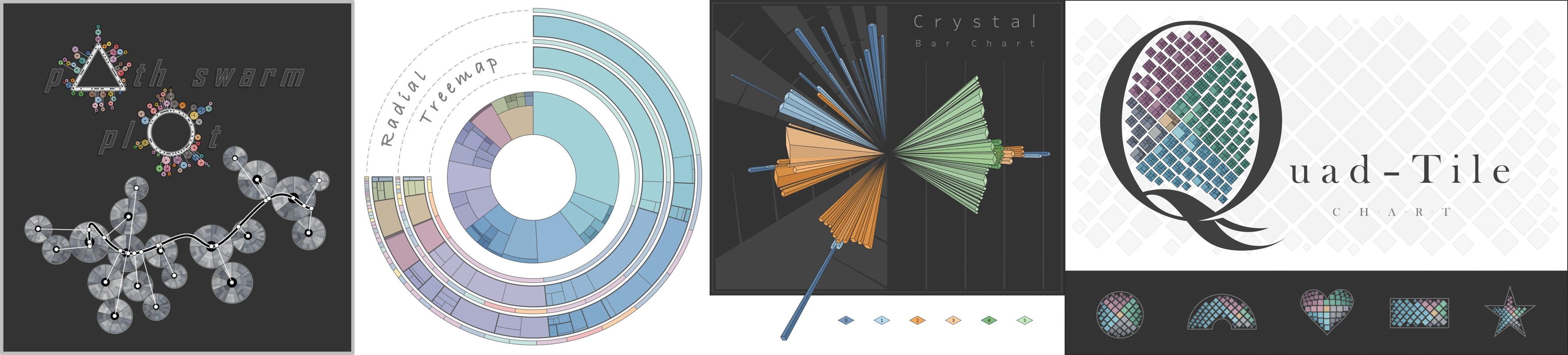
Visualization math toolkit.

Project description
vizmath
(Multichord Diagram)
Library of unique visualization algorithms. From time to time, I like to come up with fun new ways to visualize data and turn those ideas into python code!
Walkthroughs: https://towardsdatascience.com/author/nickgerend/
install
pip install vizmath
Dependencies:
pandasfor IO operationsnumpyfor computationsmatplotlibfor viz previewsscipywith .optimize, .interpolate, and .spatial for special operations
viz methods
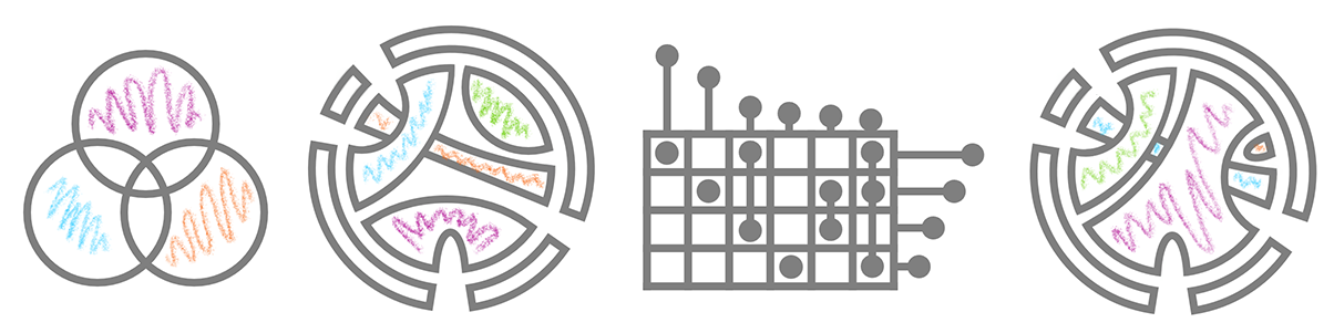
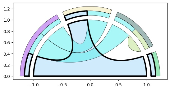
Multichord Diagram
Evolution (Venn Diagram > Chord Diagram > UpSet Plot > Multichord Diagram):
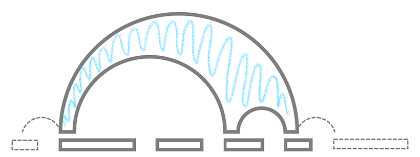
Multi-Arc Diagram Illustrating a Cartesian Layout of a Multichord:
Add multiset and set legends:
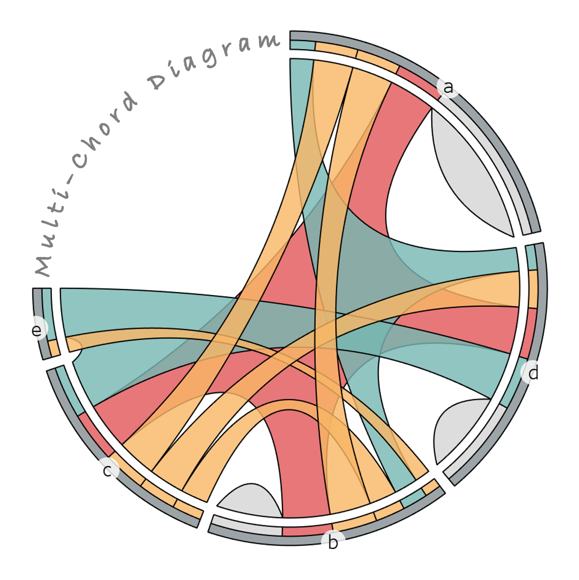
Input Data:
import pandas as pd
# setup unique multisets and their values
data = [['a,b,d', .000001], ['b,c', .000001], ['b,d', .000001], ['c', .000001]]
df = pd.DataFrame(data, columns = ['multiset', 'value'])
Multichord:
from vizmath.multichord_diagram import multichord
mc = multichord(df, multiset_field='multiset', value_field='value',
    percent=50., rotate_deg=-90)
mc.multichord_plot(level = 3, transparency = 0.5)
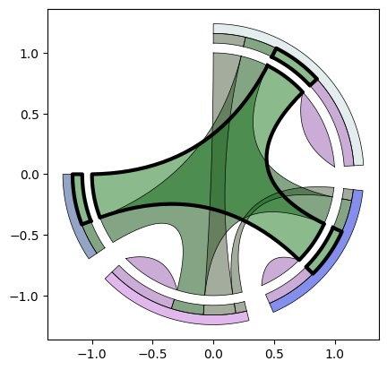
Random Multichord:
mc = multichord.random_multichord(num_sets=4, num_multisets=7, percent=75)
mc.multichord_plot(level=3)
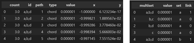
Outputs:
mc.o_multichord.df.head()
mc.upset_df.head()
Path-Swarm
Elements:
Input data:
from vizmath.path_swarm import pathswarm as ps
import pandas as pd

data = {
    'id' : [str(i) for i in range(1, 16)],
    'position' : [0.36,0.36,0.32,0.14,0.96,0.24,
        0.3,0.44,0.92,0.26,1.46,0.6,0.24,1.38,1.04],
    'size' : [1.16,1.74,0.26,0.46,0.32,0.98,0.62,
        1.84,1.96,1.98,1.22,1.86,0.6,0.92,0.78]
}
df = pd.DataFrame(data)
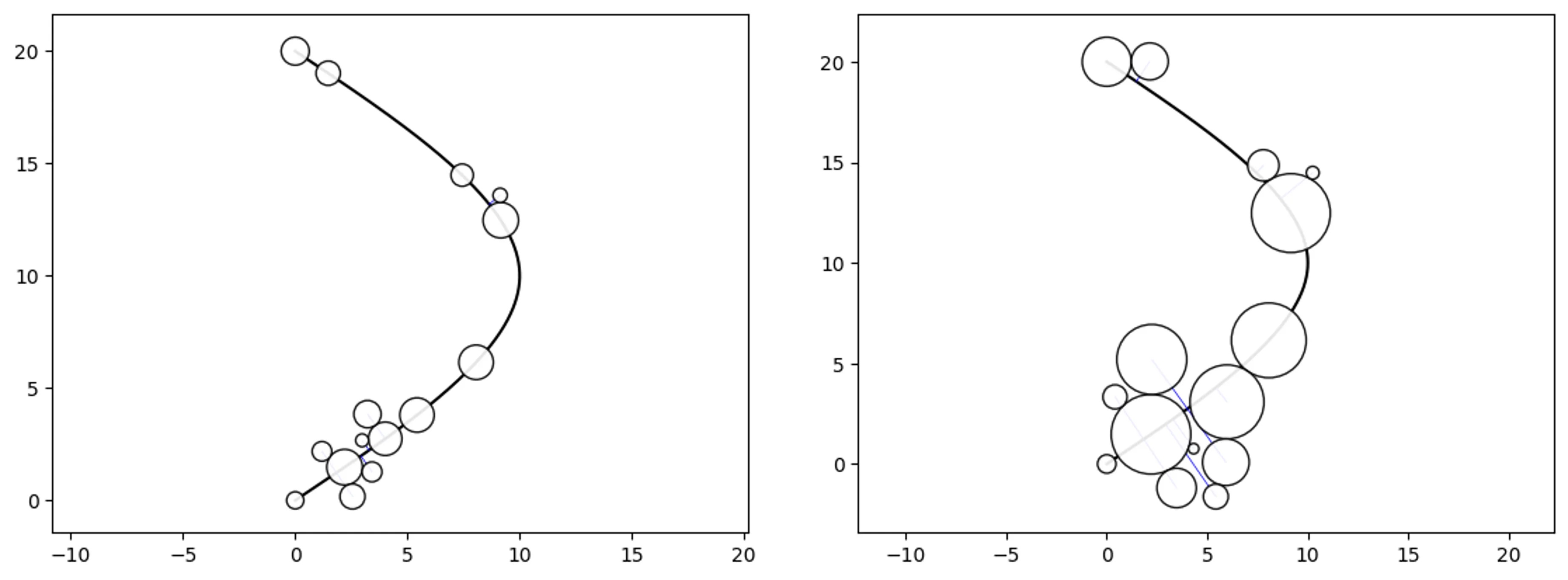
Simple Path-Swarm
# create a path and 2 path-swarm objects for different sizing
path = [(0,0),(10,10),(0,20)]
o_ps_area = ps(df=df, id_field='id', position_field='position',
    size_field='size', path=path, kwargs={'size_by':'area'})
o_ps_radius = ps(df=df, id_field='id', position_field='position',
    size_field='size', path=path, kwargs={'size_by':'radius'})

# plot the charts (sized by area and radius)
o_ps_area.plot_path_swarm()
o_ps_radius.plot_path_swarm()
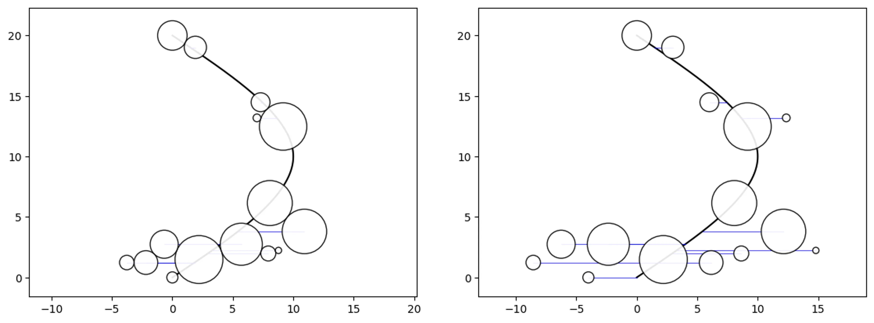
Shape-axis and Buffer properties:
o_ps_90 = ps(df=df, id_field='id', position_field='position',
    size_field='size', path=path, direction_override=90,
    kwargs={'size_by':'radius'})
o_ps_90_buffer = ps(df=df, id_field='id', position_field='position',
    size_field='size', path=path, direction_override=90,
    buffer=0.5, kwargs={'size_by':'radius'})

# plot the charts
o_ps_90.plot_path_swarm()
o_ps_90_buffer.plot_path_swarm()
Horizon and Path-offset parameters:
o_ps_top = ps(df=df, id_field='id', position_field='position',
    size_field='size', path=path,
    kwargs={'size_by':'radius', 'horizon':'top'})
o_ps_bottom = ps(df=df, id_field='id', position_field='position',
    size_field='size', path=path,
    kwargs={'size_by':'radius', 'horizon':'bottom'})
o_ps_bottom_offset = ps(df=df, id_field='id', position_field='position',
    size_field='size', path=path,
    kwargs={'size_by':'radius', 'horizon':'bottom', 'offset':-2})

# plot the charts
o_ps_top.plot_path_swarm()
o_ps_bottom.plot_path_swarm()
o_ps_bottom_offset.plot_path_swarm()
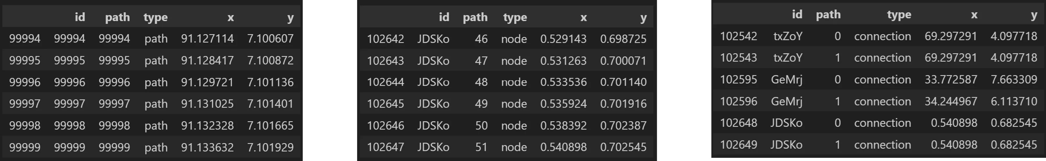
Output:
o_ps.o_pathswarm.to_dataframe()
df = o_ps.o_pathswarm.df

# now we can review a sample of each type of output
df[df['type']=='path'][-6:]
df[df['type']=='node'][-6:]
df[df['type']=='connection'][-6:]
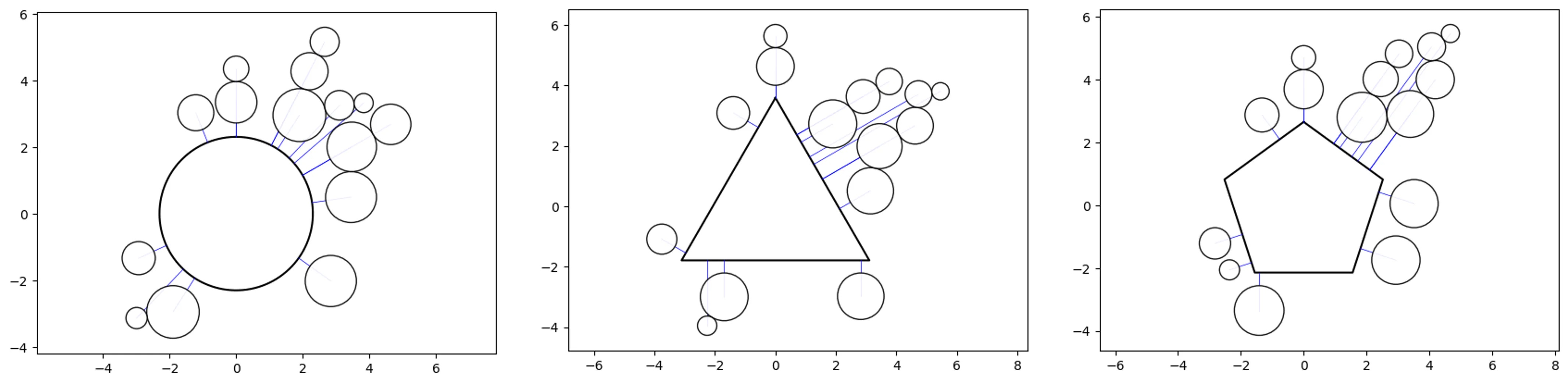
Super-Swarm:
# create a couple super swarm objects with different shapes
o_ss_circle = ss(df=df, id_field='id', position_field='position',
    size_field='size')
o_ss_triangle = ss(df=df, id_field='id', position_field='position',
    size_field='size', shape='p3')
o_ss_pentagon = ss(df=df, id_field='id', position_field='position',
    size_field='size', shape='p5')

# plot the charts
o_ss_circle.plot_super_swarm()
o_ss_triangle.plot_super_swarm()
o_ss_pentagon.plot_super_swarm()
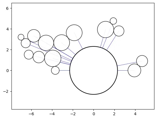
Max parameter:
# (the "min" parameter can be adjusted also)
min = df['position'].min()
delta=(df['position'].max()-df['position'].min())*2
o_ss_circle_half= ss(df=df, id_field='id', position_field='position',
    size_field='size', max=delta+min, kwargs={'offset':1}, rotation=-90)

# plot the chart
o_ss_circle_half.plot_super_swarm()
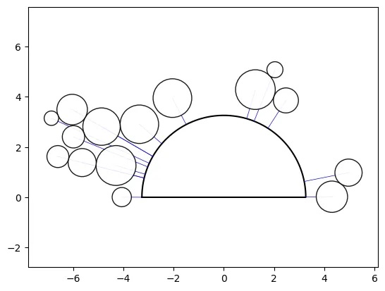
Custom Path Swarm:
# calculate the area for the central shape from the sum of the
# individual circle areas, assuming they are sized by area (deafult)
area = df['size'].sum()
# calculate the radius for an area equal to a half circle
r = (2*area/pi)**(1/2)
path = [(x,y) for x,y,_ in circle(0., 0., r=r, points=200,
    end_cap=True, spread=180)]
path.append(path[0]) # add the starting point to close the loop
offset = area/40. # add a small offset (equal to the super swarm default)
ratio = 2/pi # diameter to half circle ratio
min = df['position'].min()
delta = (df['position'].max()-df['position'].min())
# add a small offset (1e-5) for align last shape axis with the x-axis
max = min + (delta + delta*ratio) + 1e-5
# create a custom path swarm object to simulate a super swarm
o_ss_custom = ps(df=df, id_field='id', position_field='position',
    size_field='size', path=path, interp='linear', rotation=-90,
    kwargs={'horizon':'top', 'offset':offset}, max=max)

# plot the chart
o_ss_custom.plot_path_swarm()
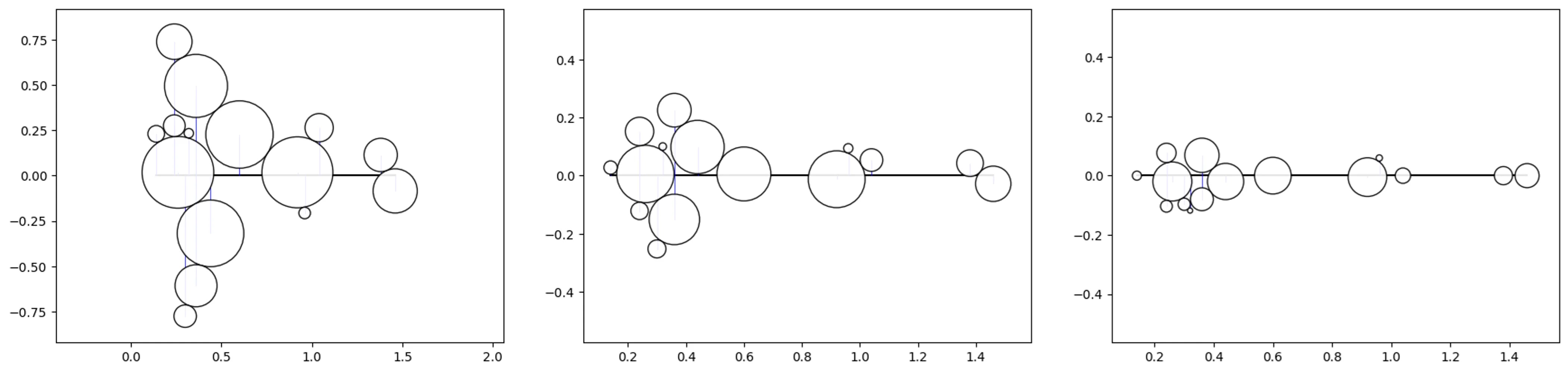
Bee-Swarm
# Let's test out 3 different sizes using the previous data
df_copy = df.copy(deep=True)
df['size'] = df_copy['size']/10 # /20, /30

# create a bee swarm object
o_bs = bs(df=df, id_field='id', position_field='position',
    size_field='size', kwargs={'size_by':'radius'})

# plot the chart (repeat for each sizing above)
o_bs.plot_bee_swarm()
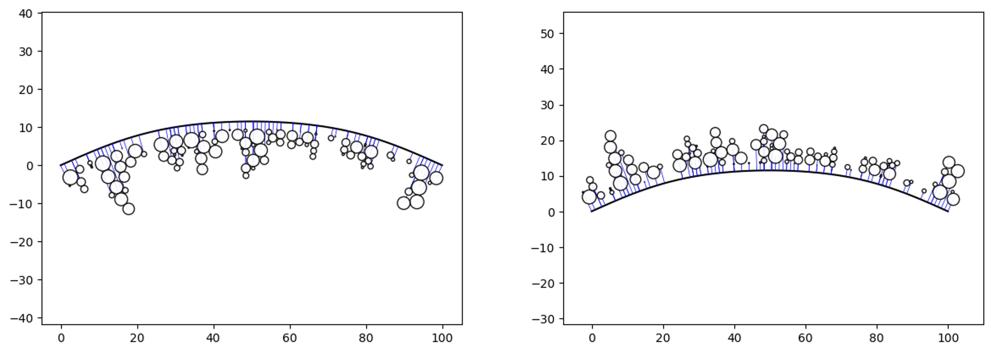
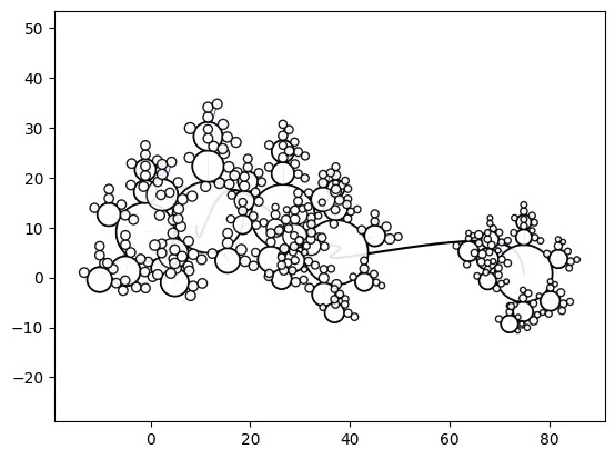
Boundary-Swarm
# create some random data and a boundary
df = ps.random_pathswarm(100).df
boundary = [(0,0),(30,10),(70,10),(100,0)]
offset = 2

# create some path swarm objects
o_ps_bottom = ps(df, 'id', 'position', size_field='size',
    path=boundary, kwargs={'horizon':'bottom',
    'size_by':'radius', 'offset':-offset})
o_ps_top = ps(df, 'id', 'position', size_field='size',
    path=boundary, kwargs={'horizon':'top',
    'size_by':'radius', 'offset':offset})

# plot the charts
o_ps_bottom.plot_path_swarm()
o_ps_top.plot_path_swarm()
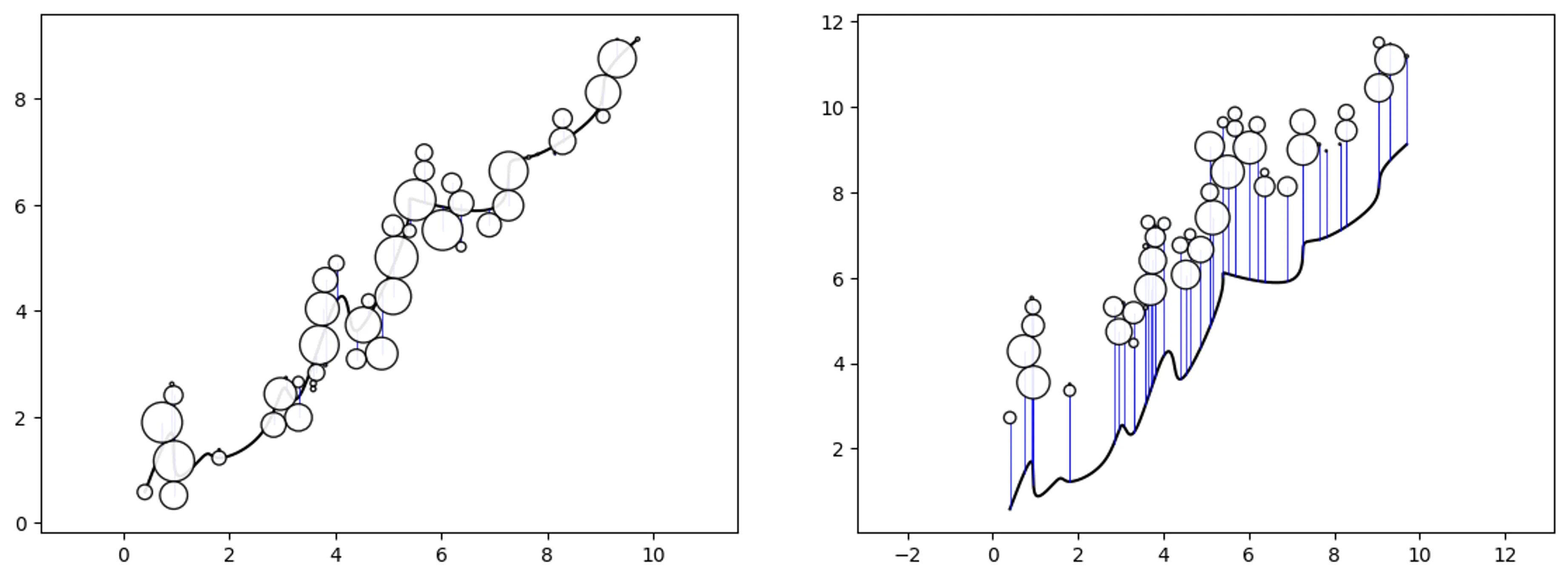
Trend-Swarm
# create some random data and a trend
df = ps.random_pathswarm(50).df
trend = [
    (0.404041, 0.582512),(0.909091, 1.697087),(1.010101, 0.910159),
    (1.515152, 1.263364),(1.818182, 1.226223),(2.626263, 1.717625),
    (3.030303, 2.546605),(3.333333, 2.413584),(3.939394, 4.031526),
    (4.242424, 4.023283),(4.545455, 3.761400),(5.353535, 5.621923),
    (5.555556, 6.075509),(6.969697, 5.934414),(7.272727, 6.727741),
    (7.777778, 6.938061),(8.888889, 7.703593),(9.090909, 8.424336),
    (9.696972, 9.124426)]

# adjust the deafault size to see the trend line better
df['event'] = df['size']/5

# create some path swarm objects
o_ps_trend = ps(df, 'id', 'position', size_field='event',
    path=trend, direction_override=0, kwargs={'size_by':'radius'})
o_ps_trend_offset = ps(df, 'id', 'position', size_field='event',
    path=trend, direction_override=0, kwargs={'size_by':'radius',
    'horizon':'top','offset':2})

# plot the charts
o_ps_trend.plot_path_swarm()
o_ps_trend_offset.plot_path_swarm()
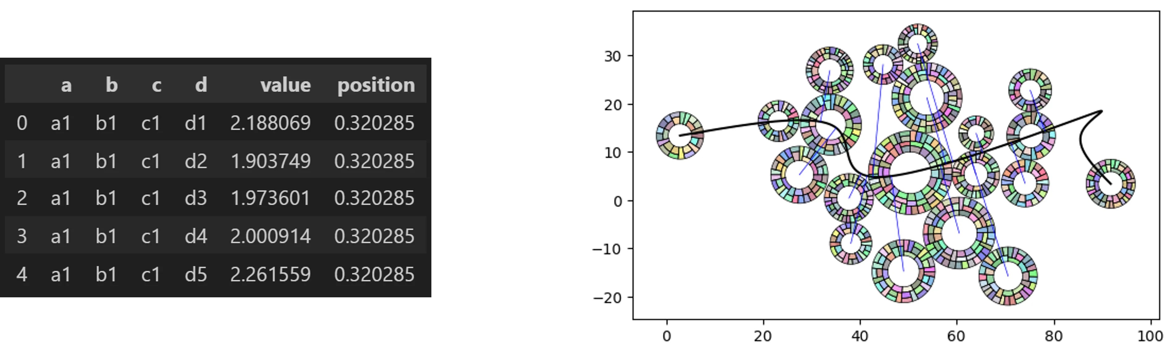
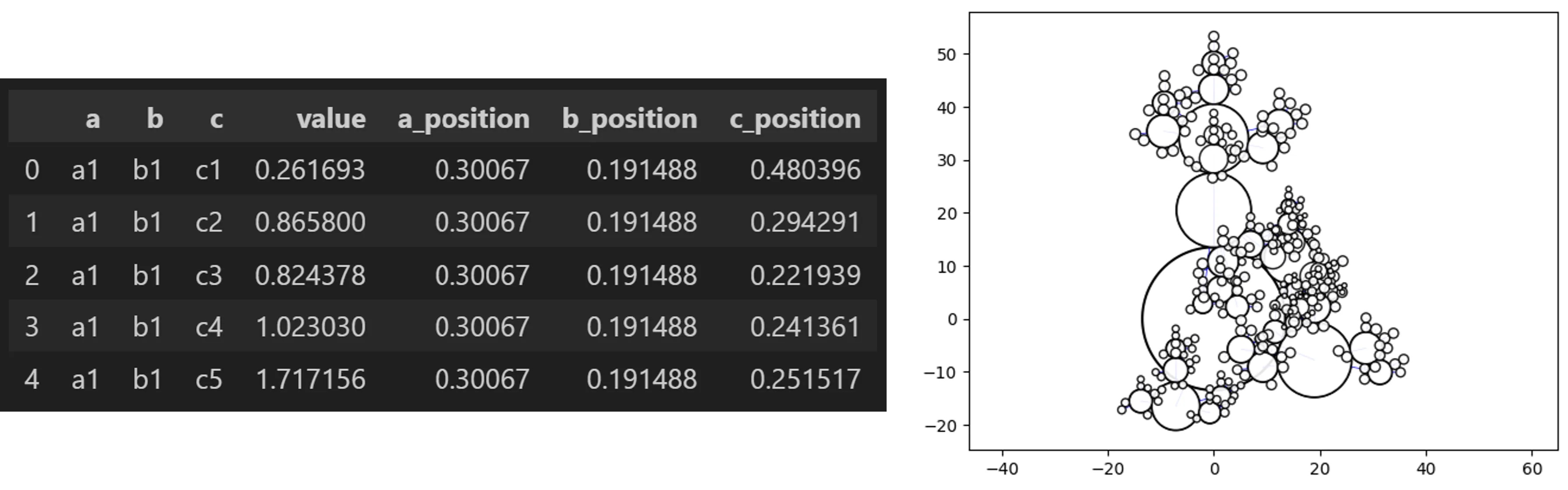
Rad-Swarm
from vizmath.path_swarm import radswarm as rs

# a Path Swarm Radial Treemap with random hierarchical dummy data
o_rs_df = rs.random_radswarm(data_only=True)
o_rs_df.head()

# now let's make a Path Swarm Radial Treemap leverging random data
# and a random path

o_rs = rs.random_radswarm()
o_rs.plot_rad_swarm()

# the underlying path swarm and radial treemap inputs can be adjusted
# as needed to initialize a normal object: o_rs = rs(inputs...)
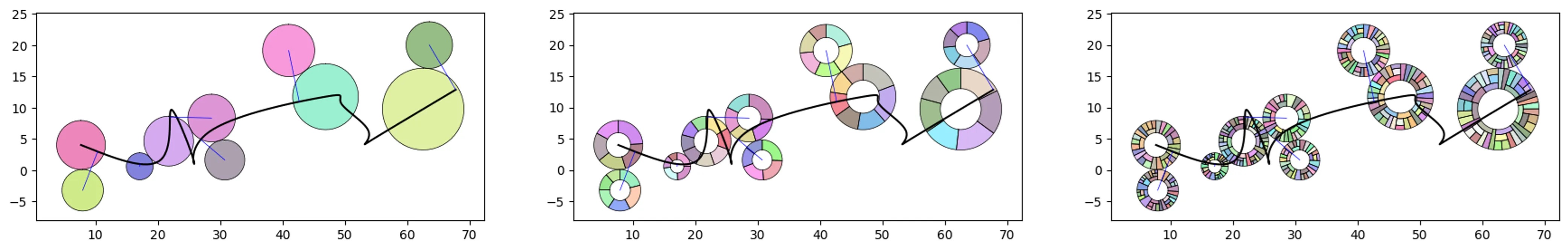
Look at each level:
# let's create a rad swarm object and plot each level
o_rs = rs.random_radswarm(10, 3, value_range_h=(.01,5),
    items_range_h=(5,8))
o_rs.plot_rad_swarm(level=1)
o_rs.plot_rad_swarm(level=2)
o_rs.plot_rad_swarm(level=3)

# rad swarm outputs:

# rad swarm data output
df_rad_swarm = o_rs.radtreemap.df_rad_treemap

# generate path swarm output
o_rs.pathswarm.o_pathswarm.to_dataframe()
df_path_swarm = o_rs.pathswarm.o_pathswarm.df
Hyper Swarm
from vizmath.path_swarm import hyperswarm as hs

# a Hyper Swarm with random hierarchical dummy data
o_hs_df = hs.random_hyperswarm(data_only=True)
o_hs_df.head()

# now let's make a Hyper Swarm leverging random data

o_hs = hs.random_hyperswarm()
o_hs.plot_hyper_swarm()

# the underlying super swarm inputs can be adjusted as needed
# to initialize a normal object: o_hs = hs(inputs...)
Hyper-Path-Swarm
o_hs = hs.random_hyperswarm(top_level_as_path=True)
o_hs.plot_hyper_swarm()
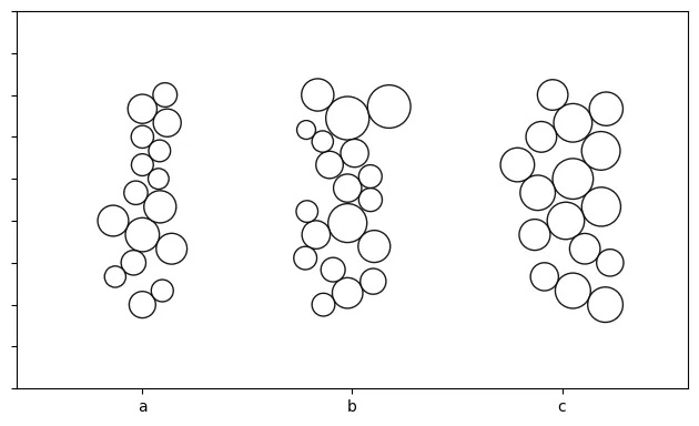
Jitter-Swarm
from vizmath.radial_treemap import rad_treemap as rt
from vizmath.path_swarm import beeswarm as bs
import numpy as np

import matplotlib.pyplot as plt
from matplotlib.patches import Circle

# let's create a function to create some dummy data
# we can utilize the hierarchical data creator from vizmath.radial_treemap
def ps_j_data(num_top_level_items, num_levels, value_range_h, sig_h,
    outlier_fraction_h, use_log_h, items_range_h, jitter_range):
    df_h = rt.random_rad_treemap(data_only=True,
        num_top_level_items=num_top_level_items,
        num_levels=num_levels, value_range=value_range_h, sig=sig_h,
        items_range=items_range_h, outlier_fraction=outlier_fraction_h,
        use_log=use_log_h)
    df_h = df_h.groupby('a').apply(
        lambda x: x.assign(position=np.linspace(jitter_range[0],
        jitter_range[1], len(x))), include_groups=False
        ).reset_index()
    return df_h

# dummy data inputs:
#   > 3 categories, 2 levels (3 categories with x items each)
#   > value range for the sizes (.1, 1)
#   > variability factor = 2(the smaller, the more variable)
#   > outliter fraction = .2, use a log transform for random values
#   > set x items for each category between (15, 20)
#   > create a jitter range (positions along the path) between (0, 5)
df = ps_j_data(3, 2, (.1,1), 2, .2, True, (15,20), (0,5))

# now we can create a bee swarm for each category and extract the plots
fig, axs = plt.subplots()
category = 0
step_size = 5
for a in df['a'].unique().tolist():
    df_ps = df[df['a']==a].copy(deep=True)
    o_ps = bs(df_ps, 'b', 'position', size_field='value',
        rotation=90, center_clusters=True)
    [setattr(n, 'node_x', n.node_x + category*step_size)
        for n in o_ps.pathswarm.nodes]
    fig_tmp, ax_tmp = o_ps.plot_bee_swarm(plot=False)
    for patch in ax_tmp.patches:
        if isinstance(patch, Circle):
            circle = Circle(patch.center, patch.radius,
                edgecolor=patch.get_edgecolor(),
                facecolor=patch.get_facecolor(),
                fill=patch.get_fill())
            axs.add_patch(circle)
    category += 1
    plt.close(fig_tmp)
axs.set_aspect('equal', 'box')
axs.set_xlim((-3,13)) # manually set for the example
axs.set_ylim((-7,2)) # manually set for the example
axs.set_xticks([0, 5, 10]) # manually set from the step size
axs.set_xticklabels(['a', 'b', 'c']) # manually set from the categories
axs.set_yticklabels([])
plt.tight_layout()
plt.show()
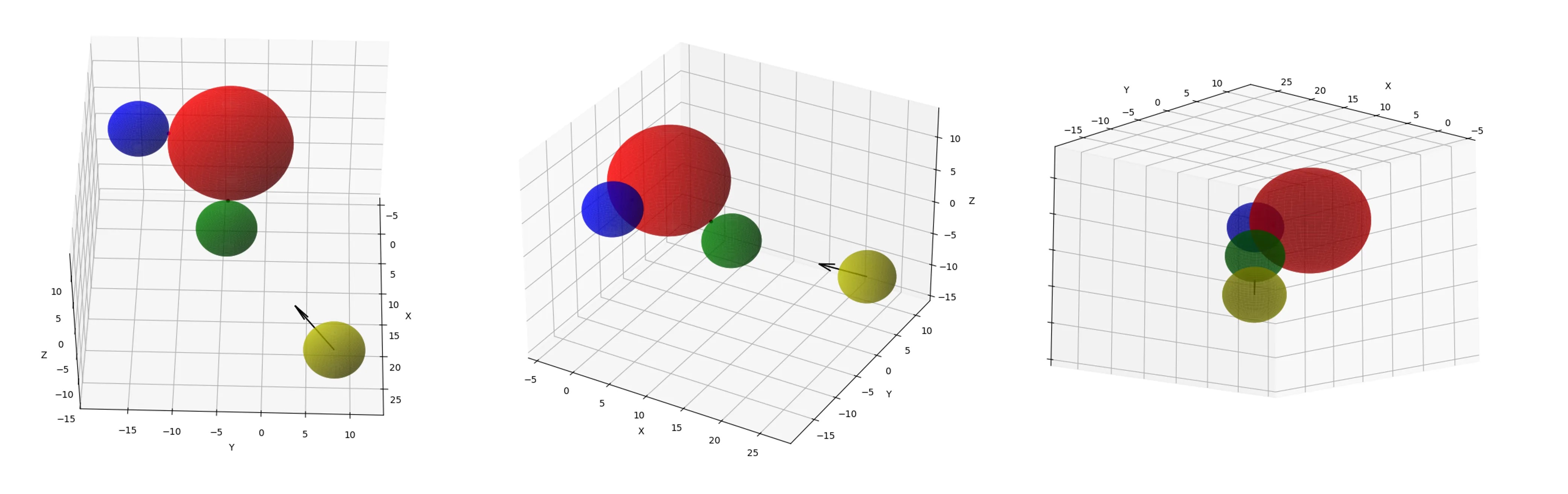
3D Swarm
import numpy as np
import matplotlib.pyplot as plt
%matplotlib qt # 3d interactive window

def check_for_collision(fx_sphere_c, fx_sphere_r,
    mv_sphere_ci, mv_sphere_r, direction_vector):
    # normalize the direction vector
    norm_direction = \
        direction_vector/np.linalg.norm(direction_vector)
    # vector from the initial position of the
    # moving sphere to the fixed sphere
    relative_position = fx_sphere_c - mv_sphere_ci
    projection_length = \
        np.dot(relative_position, norm_direction)
    # closest approach point along the direction vector
    closest_approach = \
        mv_sphere_ci+projection_length*norm_direction
    # distance from the closest approach point
    # to the fixed sphere center
    distance_to_center = \
        np.linalg.norm(closest_approach-fx_sphere_c)
    # check if the closest approach distance is
    # less than or equal to the sum of the radii
    if distance_to_center <= (fx_sphere_r+mv_sphere_r):
        return True, norm_direction
    else:
        return False, norm_direction

def calculate_final_positions(fx_sphere_c, fx_sphere_r,
    mv_sphere_ci, mv_sphere_r, norm_direction):
    # offset distance from the normal vector
    # to the moving sphere vector
    vector_to_center_dist = \
        np.linalg.norm(np.cross(norm_direction,fx_sphere_c-mv_sphere_ci))
    offset_distance = \
        np.sqrt((fx_sphere_r + mv_sphere_r)**2-vector_to_center_dist**2)
    # projection distance
    distance_to_travel_1 = \
        np.dot(fx_sphere_c-mv_sphere_ci,norm_direction)-offset_distance
    distance_to_travel_2 = \
        np.dot(fx_sphere_c-mv_sphere_ci,norm_direction)+offset_distance
    # final positions of the moving sphere on either side of
    # the fixed sphere (assuming offset_distance > 0)
    final_position_1 = mv_sphere_ci+norm_direction*distance_to_travel_1
    final_position_2 = mv_sphere_ci+norm_direction*distance_to_travel_2
    return final_position_1, final_position_2

def plot_spheres(fx_sphere_c, fx_sphere_r, mv_sphere_ci,
    mv_sphere_c1, mv_sphere_c2, mv_sphere_r,
    first_collision_point, second_collision_point,
    direction_vector, resolution=100):

    fig = plt.figure()
    ax = fig.add_subplot(111, projection='3d')

    # plot the fixed sphere
    u, v = np.mgrid[0:2*np.pi:complex(resolution),
        0:np.pi:complex(resolution)]
    x = fx_sphere_c[0] + fx_sphere_r * np.cos(u) * np.sin(v)
    y = fx_sphere_c[1] + fx_sphere_r * np.sin(u) * np.sin(v)
    z = fx_sphere_c[2] + fx_sphere_r * np.cos(v)
    ax.plot_surface(x, y, z, color='r', alpha=0.6)

    # plot initial moving sphere
    x = mv_sphere_ci[0] + mv_sphere_r * np.cos(u) * np.sin(v)
    y = mv_sphere_ci[1] + mv_sphere_r * np.sin(u) * np.sin(v)
    z = mv_sphere_ci[2] + mv_sphere_r * np.cos(v)
    ax.plot_surface(x, y, z, color='y', alpha=0.6)

    # plot final moving sphere (first position)
    x = mv_sphere_c1[0] + mv_sphere_r * np.cos(u) * np.sin(v)
    y = mv_sphere_c1[1] + mv_sphere_r * np.sin(u) * np.sin(v)
    z = mv_sphere_c1[2] + mv_sphere_r * np.cos(v)
    ax.plot_surface(x, y, z, color='g', alpha=0.6)

    # plot final moving sphere (second position)
    x = mv_sphere_c2[0] + mv_sphere_r * np.cos(u) * np.sin(v)
    y = mv_sphere_c2[1] + mv_sphere_r * np.sin(u) * np.sin(v)
    z = mv_sphere_c2[2] + mv_sphere_r * np.cos(v)
    ax.plot_surface(x, y, z, color='b', alpha=0.6)

    # plot collision points where the surfaces touch
    ax.scatter(*first_collision_point, color='k', s=10)
    ax.scatter(*second_collision_point, color='m', s=10)

    # plot direction vector
    ax.quiver(mv_sphere_ci[0], mv_sphere_ci[1],
        mv_sphere_ci[2], direction_vector[0], direction_vector[1],
        direction_vector[2], color='k',
        length=2*mv_sphere_r, normalize=True)

    ax.set_xlabel('X')
    ax.set_ylabel('Y')
    ax.set_zlabel('Z')

    plt.show()

# sample data, placing one (moving) sphere relative to another (fixed)
fx_sphere_c = np.array([3.2, -4.1, 5.3]) # fixed sphere center
fx_sphere_r = 7.2 # fixed sphere radius
mv_sphere_ci = np.array([23.2, 8.1, -10.4]) # moving sphere center
mv_sphere_r = 3.5 # moving sphere radius
direction_vector = np.array([-1.1, -1.2, 0.9]) # shape axis vector

# check for collision
collision_exists, norm_direction = \
    check_for_collision(fx_sphere_c, fx_sphere_r, mv_sphere_ci,
        mv_sphere_r, direction_vector)

if collision_exists:
    # calculate the final positions of the moving sphere
    mv_sphere_c1, mv_sphere_c2 = \
        calculate_final_positions(fx_sphere_c, fx_sphere_r,
            mv_sphere_ci, mv_sphere_r, norm_direction)
    # test placement (distance between centers should equal sum of radii)
    dist_after_collision = np.linalg.norm(mv_sphere_c1 - fx_sphere_c)

    # calculate the first collision point
    first_collision_point_surface = fx_sphere_c + \
        ((mv_sphere_c1-fx_sphere_c)*fx_sphere_r/dist_after_collision)

    # calculate the second collision point
    second_collision_point_surface = fx_sphere_c + \
        ((mv_sphere_c2-fx_sphere_c)*fx_sphere_r/dist_after_collision)

    # plot the spheres
    plot_spheres(fx_sphere_c, fx_sphere_r, mv_sphere_ci, mv_sphere_c1,
        mv_sphere_c2, mv_sphere_r, first_collision_point_surface,
        second_collision_point_surface, direction_vector)

    # print inputs and outputs
    print('First Moving Sphere Center:', mv_sphere_c1.tolist())
    print('Second Moving Sphere Center:', mv_sphere_c2.tolist())
    print('Distance After Collision:', dist_after_collision)
    print('Sum of Radii:', fx_sphere_r + mv_sphere_r)
else:
    print('No collision detected.')
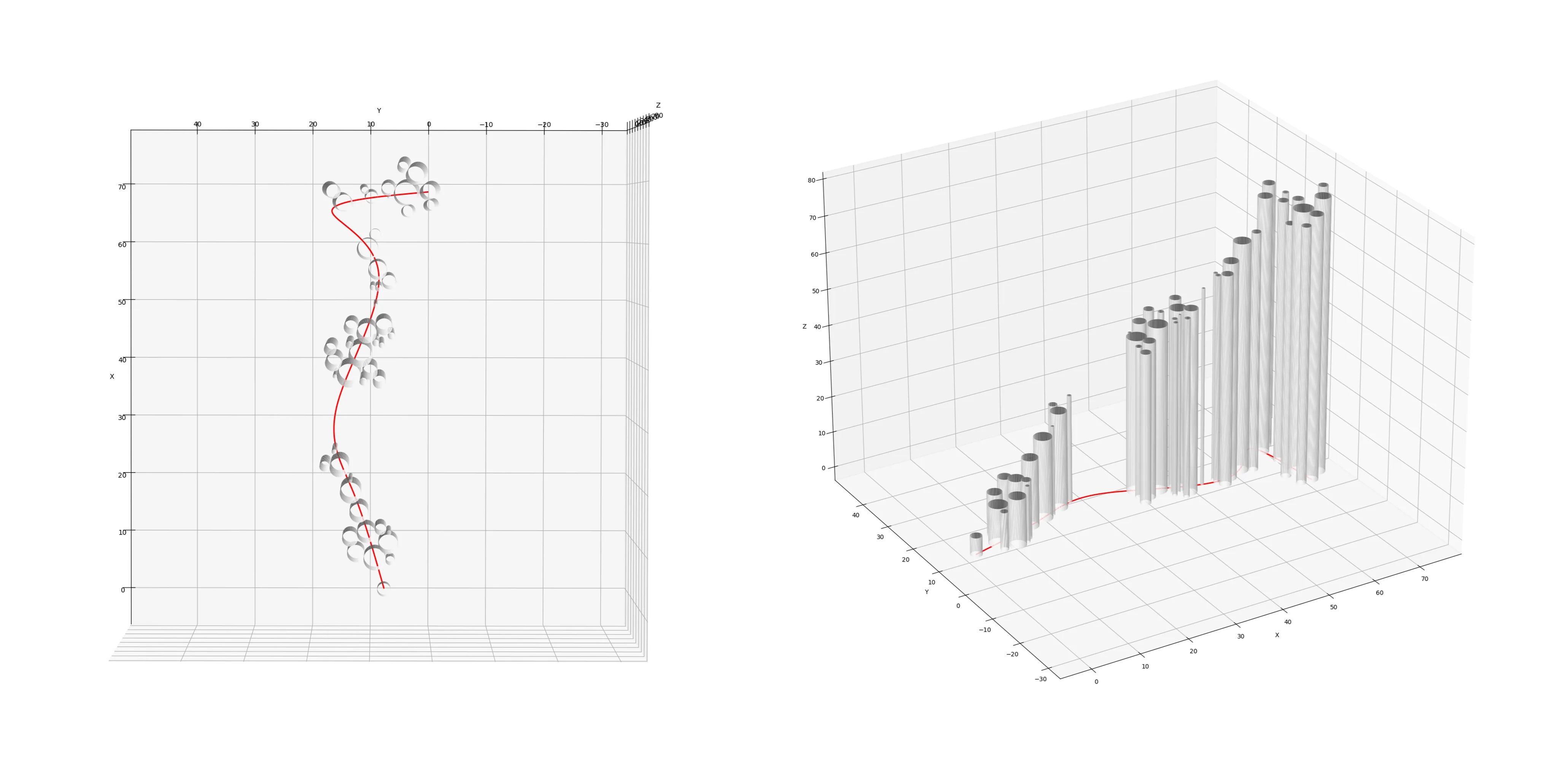
3D Path-Swarm projection
import matplotlib.pyplot as plt
import numpy as np
%matplotlib qt

def plot_cylinder(ax, x_center, y_center, radius, height, resolution=100):
    z = np.linspace(0, height, 2)
    theta = np.linspace(0, 2 * np.pi, resolution)
    theta_grid, z_grid = np.meshgrid(theta, z)
    x_grid = x_center + radius * np.cos(theta_grid)
    y_grid = y_center + radius * np.sin(theta_grid)
    ax.plot_surface(x_grid, y_grid, z_grid, color='w', alpha=0.9)

def set_axes_equal(ax):
    x_limits = ax.get_xlim3d()
    y_limits = ax.get_ylim3d()
    z_limits = ax.get_zlim3d()
    x_range = abs(x_limits[1] - x_limits[0])
    y_range = abs(y_limits[1] - y_limits[0])
    z_range = abs(z_limits[1] - z_limits[0])
    max_range = max([x_range, y_range, z_range])
    x_middle = np.mean(x_limits)
    y_middle = np.mean(y_limits)
    z_middle = np.mean(z_limits)
    ax.set_xlim3d([x_middle - max_range / 2, x_middle + max_range / 2])
    ax.set_ylim3d([y_middle - max_range / 2, y_middle + max_range / 2])
    ax.set_zlim3d([z_middle - max_range / 2, z_middle + max_range / 2])

# collect the node information
x, y, r = zip(*[(n.node_x, n.node_y, n.node_radius)
    for n in o_ps_elevation.nodes])

# collect the path information
path_x, path_y = zip(*o_ps_elevation.i_path)
path_z = [0 for _ in range(len(path_x))]

# plot path and cylinders
fig = plt.figure()
ax = fig.add_subplot(111, projection='3d')
ax.plot(path_x, path_y, path_z, color='r', linewidth=2)
for i in range(len(x)): # reuse x as a proxy for elevation
    plot_cylinder(ax, x[i], y[i], r[i], x[i]+5)
ax.set_xlabel('X')
ax.set_ylabel('Y')
ax.set_zlabel('Z')
set_axes_equal(ax)
plt.show()
Radial-Treemaps
Layouts:
Simple Radial-Treemap:
from vizmath import rad_treemap as rt
import pandas as pd
# using the example data from above:
data = [
['a1', 'b1', 'c1', 12.3],
['a1', 'b2', 'c1', 4.5],
['a2', 'b1', 'c2', 32.3],
['a1', 'b2', 'c2', 2.1],
['a2', 'b1', 'c1', 5.9],
['a3', 'b1', 'c1', 3.5],
['a4', 'b2', 'c1', 3.1]]
df = pd.DataFrame(data, columns = ['a', 'b', 'c', 'value'])
# create a rad_treemap object
# > df: DataFrame with 1 or more categorical columns of data
# and an optional 'value' column for the areas
# (otherwise groups counts are used for areas)
# > groupers: group-by columns
# > value: optional value column
# > r1, r2: inner and outer radius positions
# > a1, a2: start and end angle positions
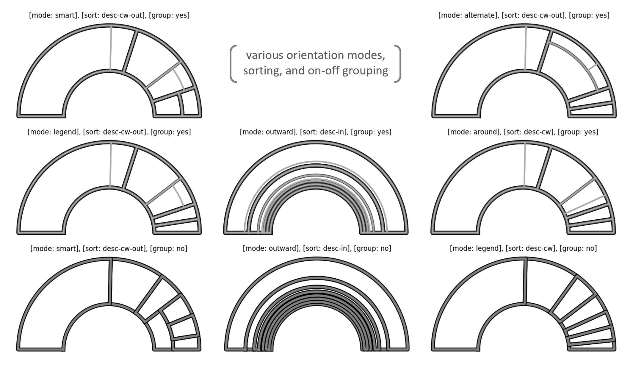
# > rotate_deg: overall rotation around the center
# > mode: container orientation method
# > other options: 'points', 'default_sort', 'default_sort_override',
# 'default_sort_override_reversed', 'mode', 'no_groups', 'full'
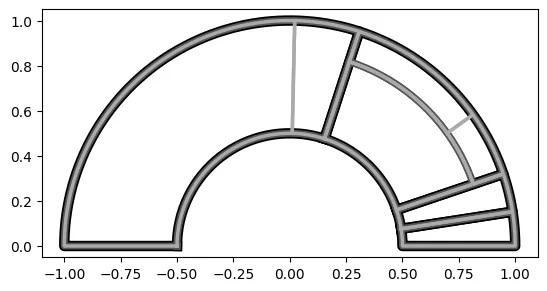
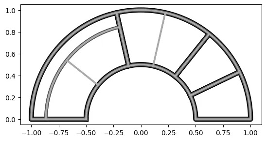
rt_1 = rt(df=df, groupers=['a','b','c'], value='value', r1=0.5, r2=1,
a1=0, a2=180, rotate_deg=-90, mode='alternate')
# plot the Radial Treemap
rt_1.plot_levels(level=3, fill='w')
Output:
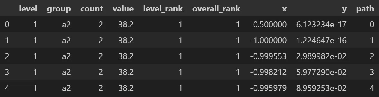
# sample the Radial Treemap DataFrame
rt_1.to_df()[['level','group','count','value',
    'level_rank','overall_rank','x','y','path']].head()
By counts:
# set 'value' to None or just leave it out since None is the default
# doing this sets the areas equal to the group counts
# in this case, each count will be one since there are no duplicates

rt_2 = rt(df=df, groupers=['a','b','c'], value=None, r1=0.5, r2=1,
  a1=0, a2=180, rotate_deg=-90, mode='alternate')

# plot the Radial Treemap
rt_2.plot_levels(level=3, fill='w')
Crystal-Bar
Elements:
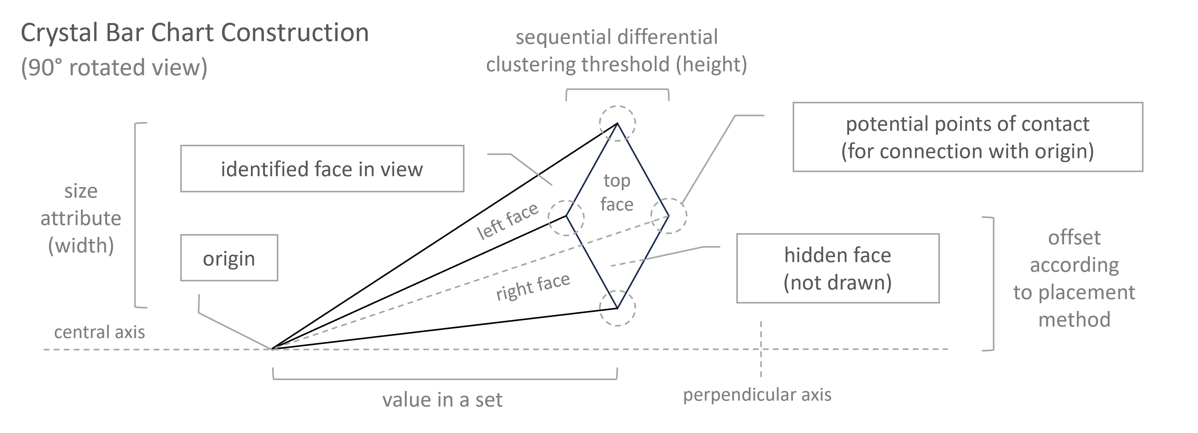
Sequential Differential Clustering:
sequence: [ 0 , 1 , 1 , 2 , 3 , 5 , 8 , 13 , 21 , 34 , 55 , 89 , 144 ]
val to val diff: [ _ , _ , 0 , 1 , 1 , 2 , 3 , 5 , 8 , 13 , 21 , 34 , 55 ]
threshold val: 5
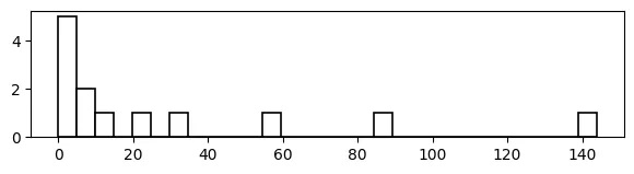
With a Histogram:
# pandas histogram
import pandas as pd
import numpy as np
data = {'value' : [0,1,1,2,3,5,8,13,21,34,55,89,144]}
df = pd.DataFrame(data=data)
data_range = df['value'].max() - df['value'].min()
num_bins = np.ceil(data_range/5).astype(int)
print(num_bins) # 29
df['value'].hist(bins=num_bins, color='w', edgecolor='black',
  linewidth=1.2, grid=False, figsize=(7,1.5))
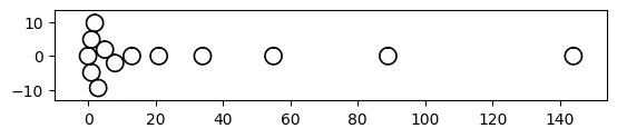
With a Bee-Swarm:
# vizmath (modified) beeswarm chart
from vizmath.beeswarm import swarm
from math import pi
data = {
    'id' : [str(i) for i in range(1, 14)],
    'value' : [0,1,1,2,3,5,8,13,21,34,55,89,144]
}
df = pd.DataFrame(data=data)
bs = swarm(df, 'id', 'value', None, size_override=pi*(5/2)**2)
bs.beeswarm_plot(color=False)
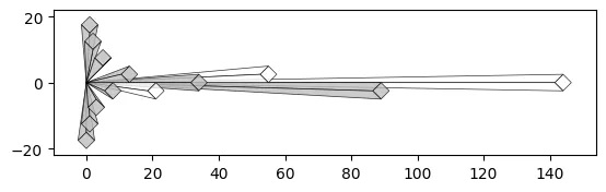
With a Crystal Bar Chart:
# vizmath crystal bar chart
from vizmath.crystal_bar_chart import crystals
data = {
    'id' : [str(i) for i in range(1, 14)],
    'value' : [0,1,1,2,3,5,8,13,21,34,55,89,144]
}
df = pd.DataFrame(data=data)
cbc = crystals(df, 'id', 'value', 5, width_override=5, rotation=90)
cbc.cbc_plot(legend=False, alternate_color=True, color=False)
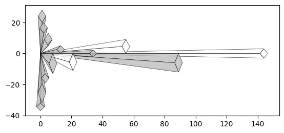
Size property:
# vizmath crystal bar chart with added width property
cbc = crystals(df, 'id', 'value', 5, width_field='size', rotation=90)
cbc.cbc_plot(legend=False, alternate_color=True, color=False)
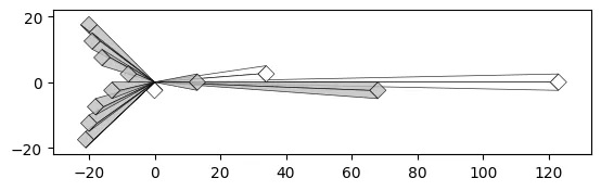
Offset property:
# vizmath crystal bar chart with adjusted origin
cbc = crystals(df, 'id', 'value', 5, width_override=5,
    rotation=90, offset=21) # new offset
cbc.cbc_plot(legend=False, alternate_color=True, color=False)
Clusters:
Containers:
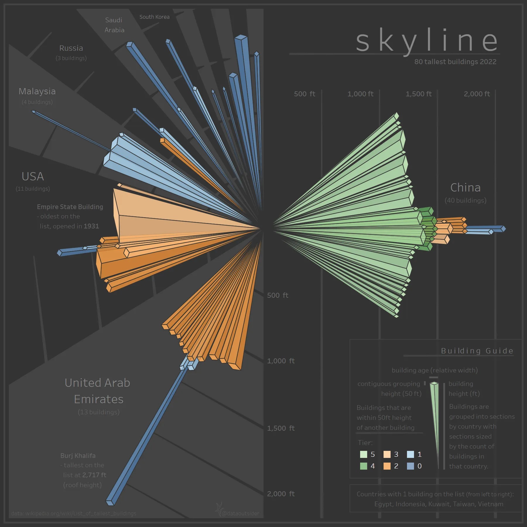
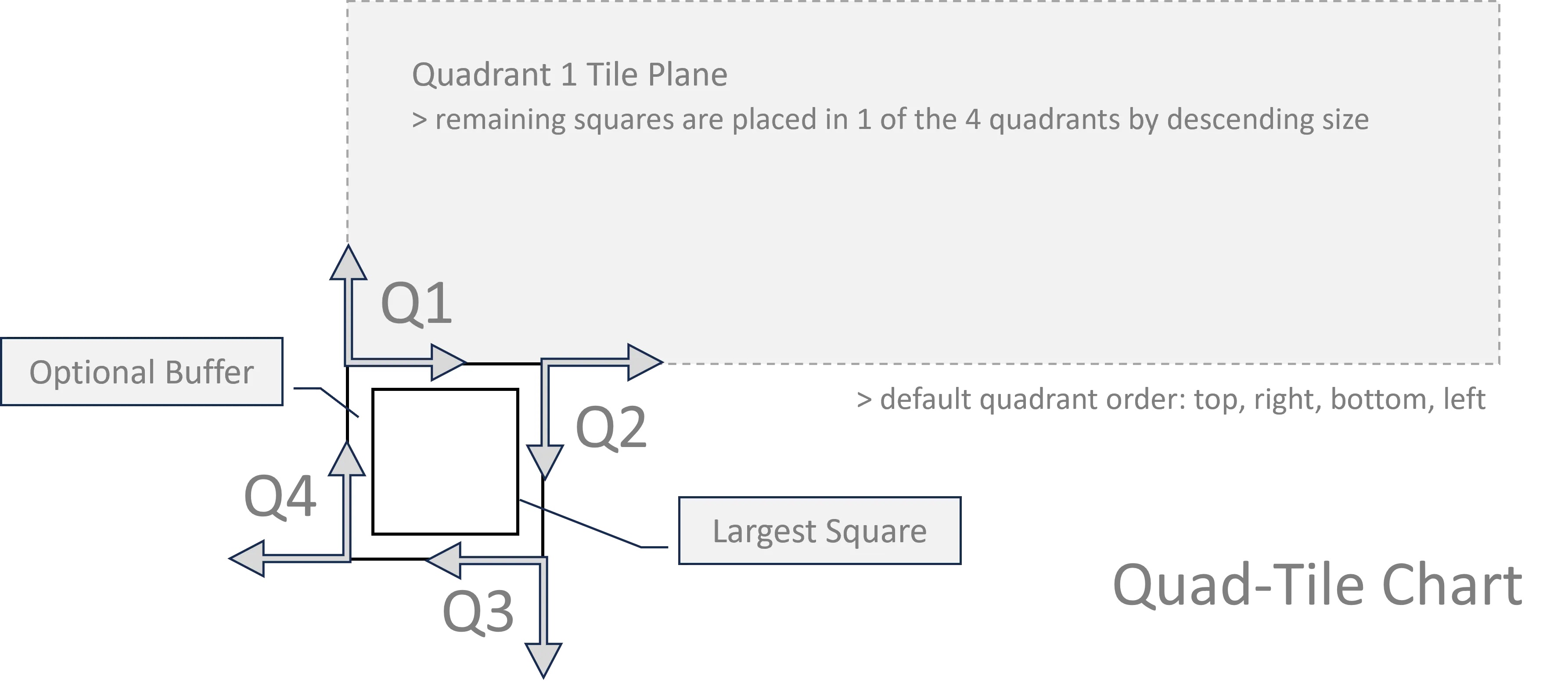
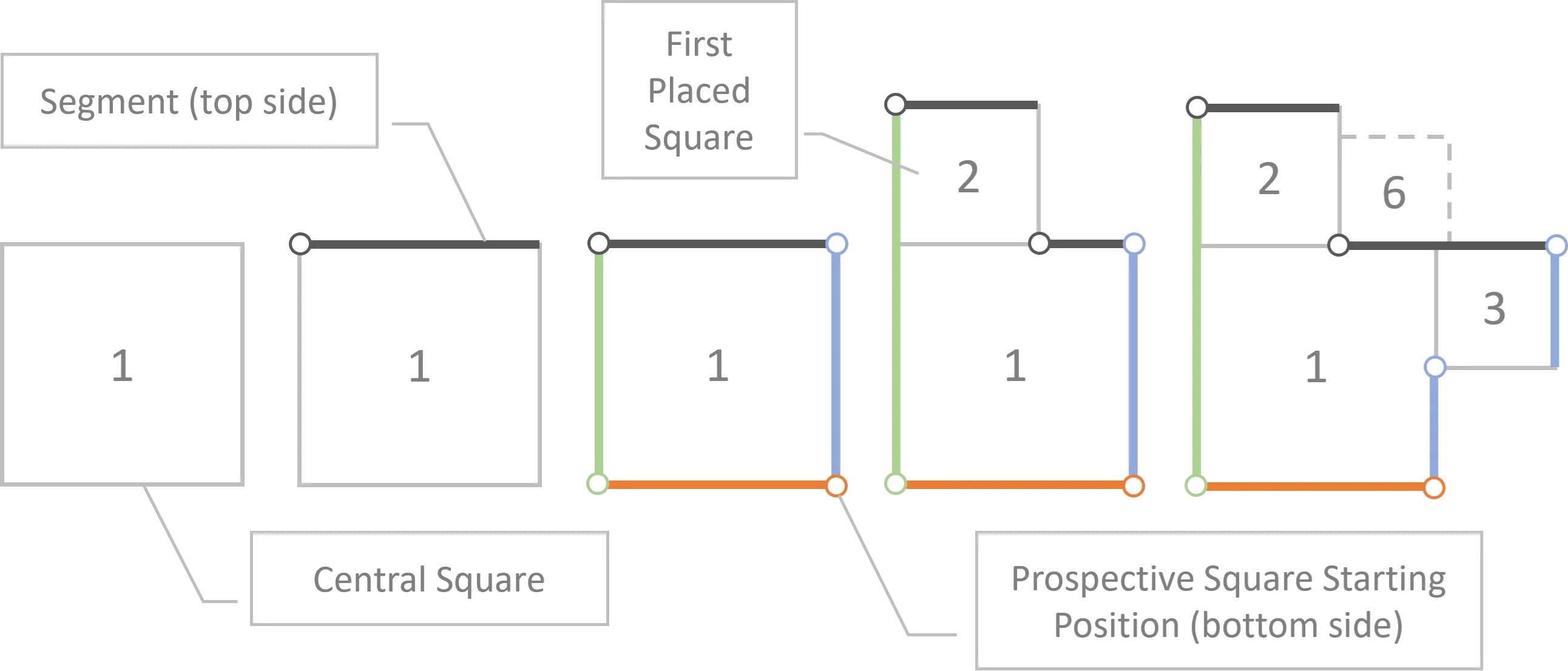
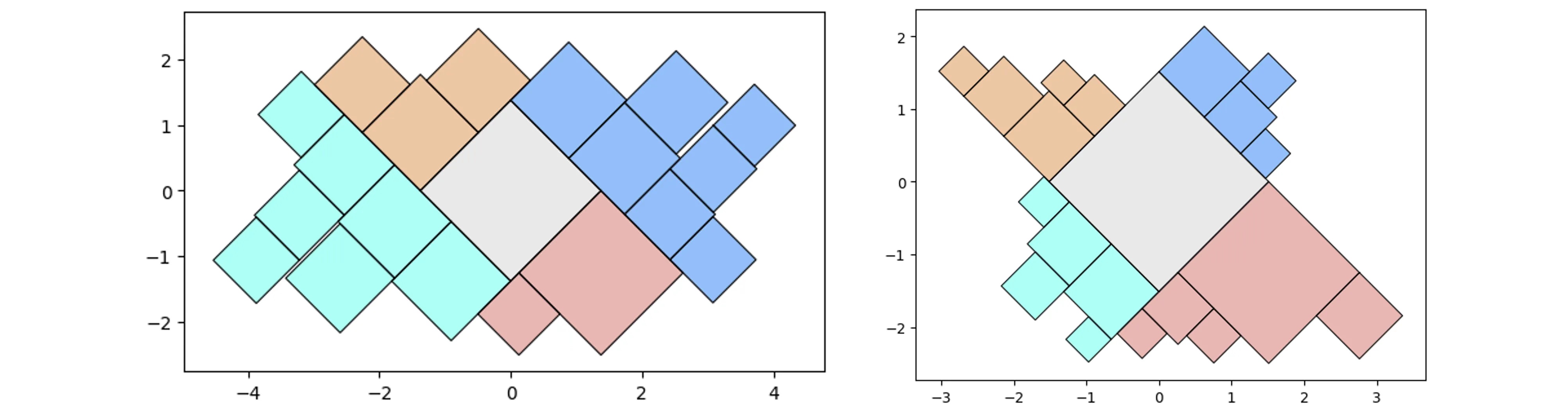
Quad-Tile
My initial approach (V1) didn’t consider a container, where the new approach (V2) does.
Quad-Tile V1
V1 Concept:
V1 Elements:
V1 Layouts:
V1 Example:
# Quad-Tile Chart v1
from vizmath.quadtile_chart import quadtile as qt
import pandas as pd

data = {
    'id' : [str(i) for i in range(1, 21)],
    'speed' : [242,200,105,100,100,95,92.5,88,80,79,
        75,67.85,61.06,60,56,55,55,55,50,50]
}
df = pd.DataFrame(data)

# create a quadtile object
#   > df: DataFrame with 1 numerical column of data and an id field
#   > id_field: required identifier field (can be dummy values)
#   > value_field: required value column
#   > xo: x-axis origin
#   > yo: y-axis origin
#   > packing: packing method ('auto','inc','num','max','min')
#   > overflow: integer threshold for 'num','max','min' packing
#   > buffer: additive value for buffering a square's size
#   > rotate: degrees to rotate the chart by
#   > constraints: polygon to encourage growth inside the perimeter
#   > size_by: 'area' or 'width'
#   > poly_sort: enable/disable sorting polygon vertices (True, False)
qt_o_area = qt(df,'id','speed', size_by='area', buffer=0)
qt_o_width = qt(df,'id','speed', size_by='width', buffer=0)

# plot the charts (sized by area and width)
qt_o_area.quadtile_plot(color='quad', cw=0.75, opacity=.9)
qt_o_width.quadtile_plot(color='quad', cw=0.75, opacity=.9)
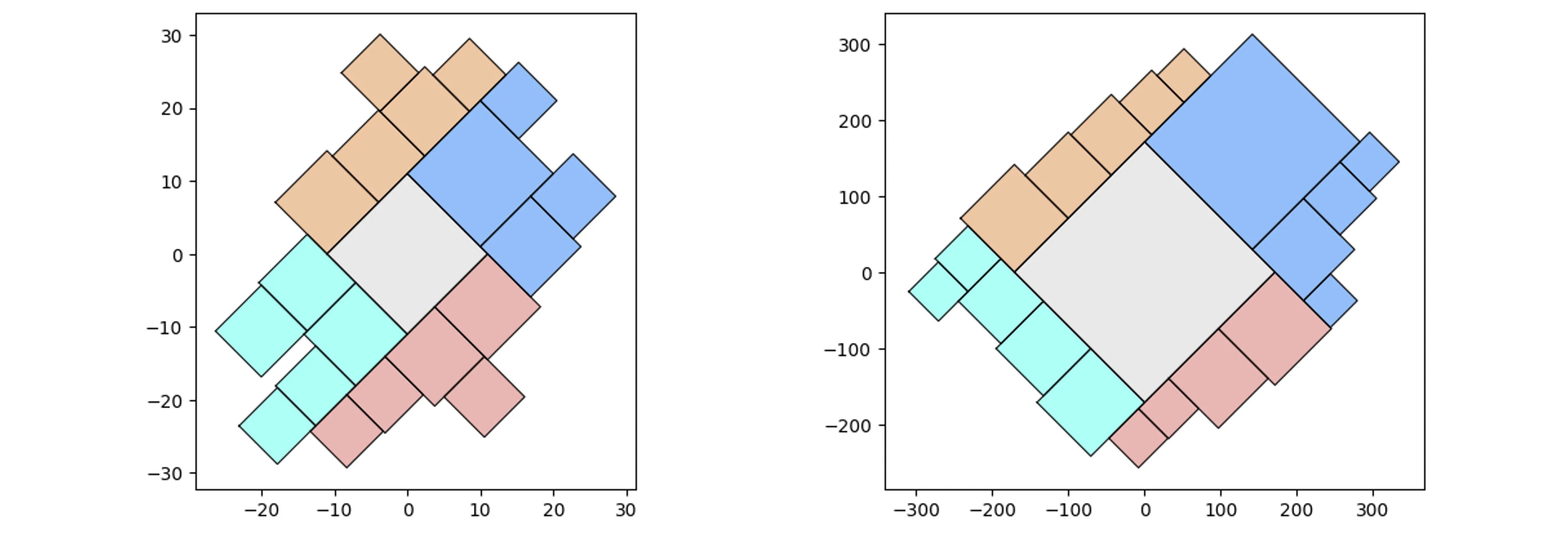
Quad-Tile V2
V2 Elements:
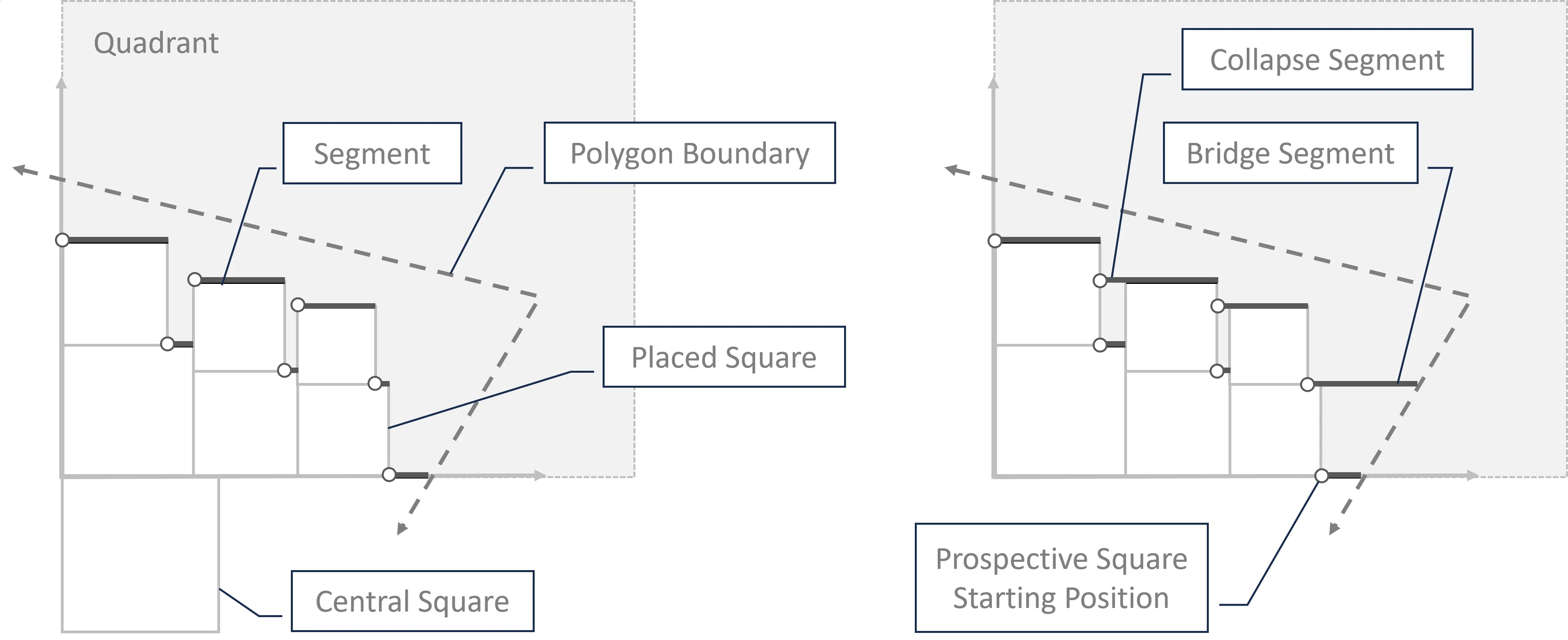
V2 Layouts:
V2 Example:
# Quad-Tile Chart v2
from vizmath.quadtile_chart import polyquadtile as pqt
import pandas as pd

data = {
    'id' : [str(i) for i in range(1, 21)],
    'speed' : [242,200,105,100,100,95,92.5,88,80,79,
        75,67.85,61.06,60,56,55,55,55,50,50]
}
df = pd.DataFrame(data)

# create a quadtile object
#   > df: DataFrame with 1 numerical column of data and an id field
#   > id_field: required identifier field (can be dummy values)
#   > value_field: required value column
#   > xo: x-axis origin
#   > yo: y-axis origin
#   > buffer: additive value for buffering a square's size
#   > rotate: degrees to rotate the chart by
#   > sides: select sides to include ('top','right','bottom','left')
#   > collapse: enable/disable collapse (True, False)
#   > constraints: polygon container to pack
#   > xc: x-axis container offset value
#   > yc: y-axis container offset value
#   > size_by: 'area' or 'width'
#   > auto: enable/disable automatic packing (True, False)
#   > auto_max_iter: iterations for automatic packing
#   > auto_min_val: minimum multiplier for automatic packing
#   > auto_max_val: maximum multiplier for automatic packing
#   > poly_sort: enable/disable sorting polygon vertices (True, False)
pqt_o_area = pqt(df,'id','speed', size_by='area', buffer=0)
pqt_o_width = pqt(df,'id','speed', size_by='width', buffer=0)

# plot the charts (sized by area and width)
pqt_o_area.polyquadtile_plot(color='quad', cw=0.75, opacity=.9)
pqt_o_width.polyquadtile_plot(color='quad', cw=0.75, opacity=.9)
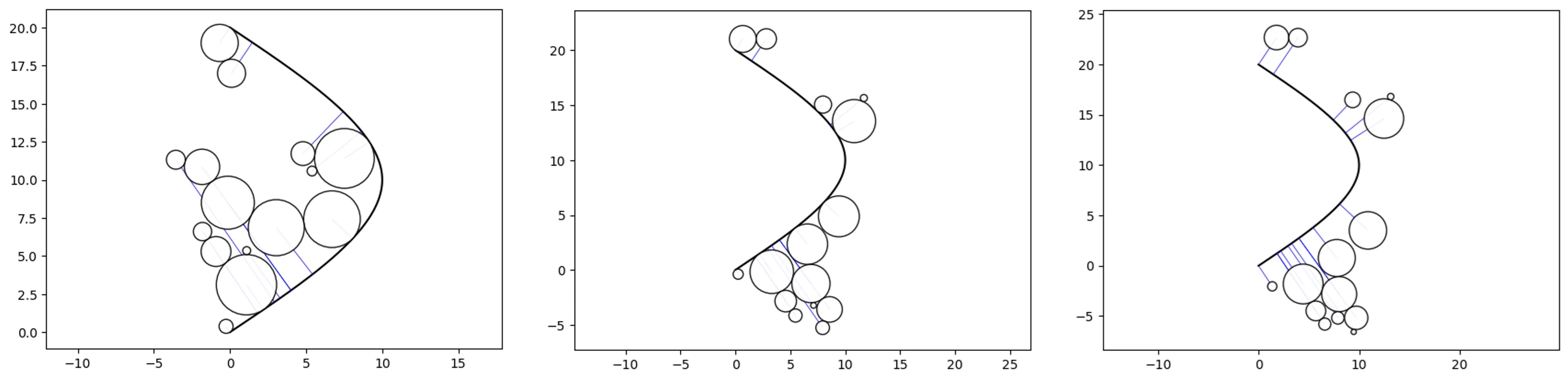
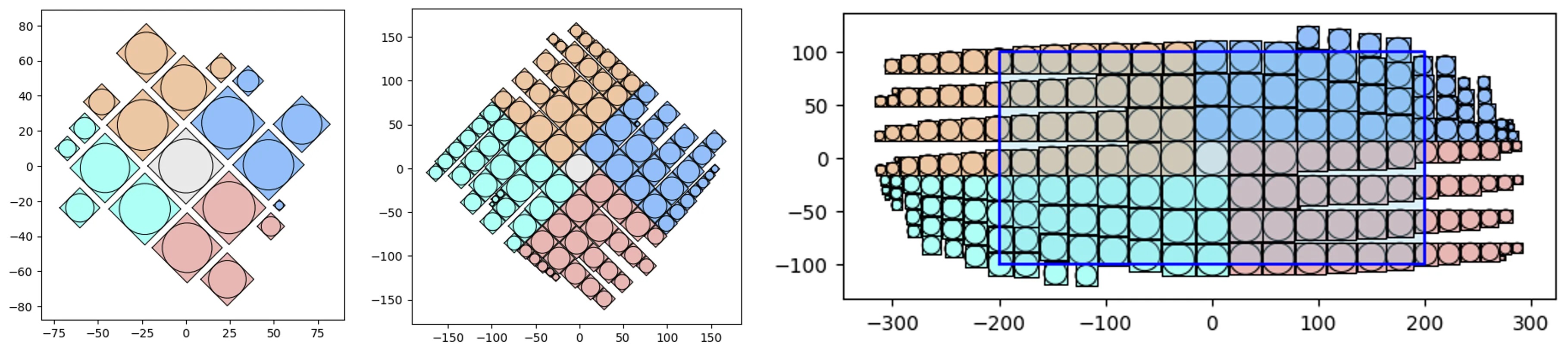
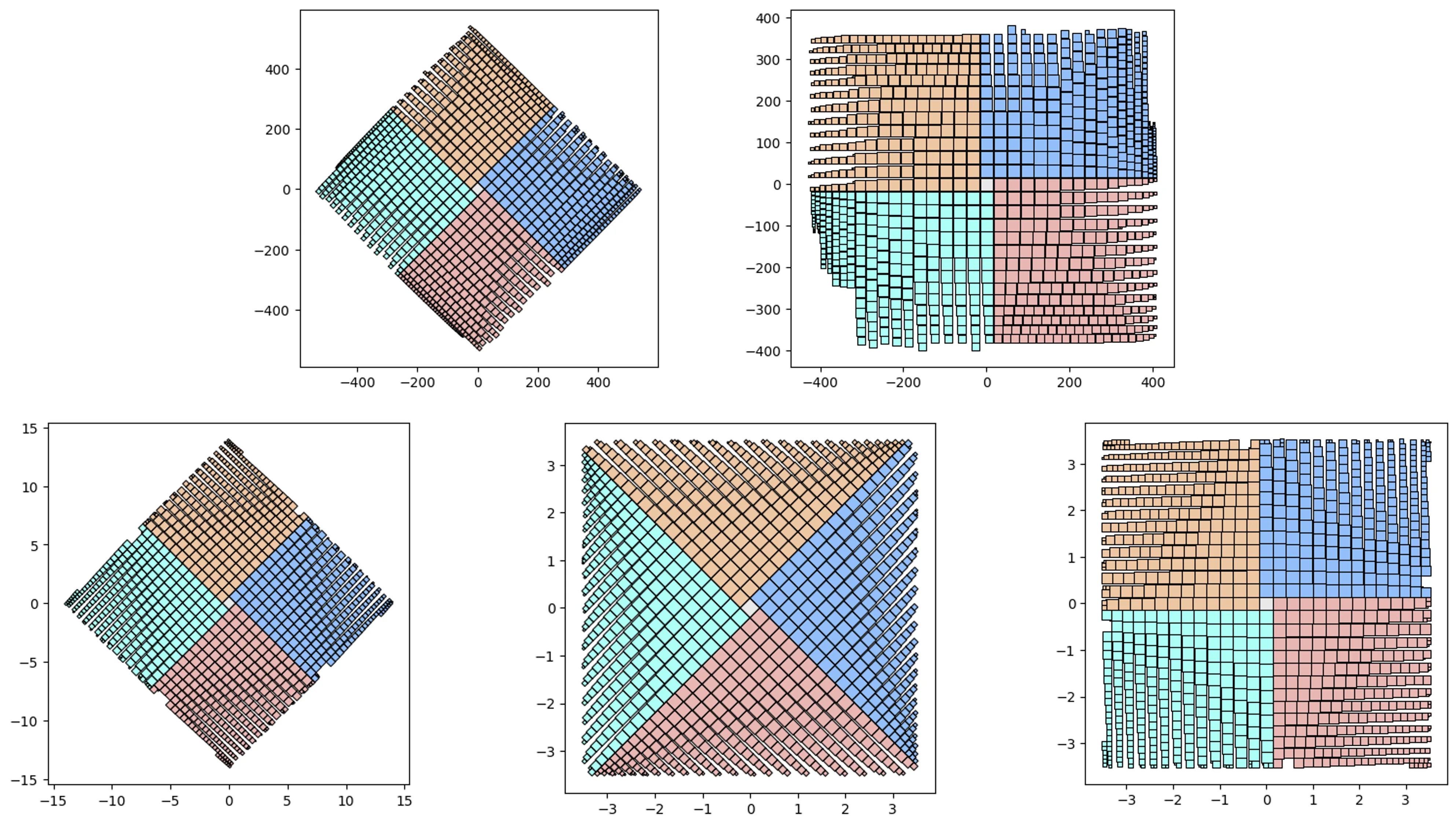
V1 vs V2 and simple containers:
# let's test 1000 randomly sized squares:
from vizmath.quadtile_chart import quadtile as qt
from vizmath.quadtile_chart import polyquadtile as pqt

# Quad-Tile Chart v1 that's rotated (top left below)
qt_o1 = qt.random_quadtile(1000, rotate=45)
qt_o1.quadtile_plot(color='quad', cw=0.75, opacity=.9)

# Quad-Tile Chart v1 that's not rotated (top right below)
qt_o2 = qt.random_quadtile(1000, rotate=0)
qt_o2.quadtile_plot(color='quad', cw=0.75, opacity=.9)

# Quad-Tile Chart v2 with a square container (bottom left below)
poly = [(-10,-10),(-10,10),(10,10),(10,-10)] # polygon container
pqt_o1 = pqt.random_polyquadtile(1000, constraints=poly, buffer=0)
pqt_o1.polyquadtile_plot(color='quad', cw=0.75, opacity=.9)

# Quad-Tile Chart v2 with a rotated aspect ratio of 1:1 (middle below)
pqt_o2 = pqt.random_polyquadtile(1000, constraints=[(1,1)], buffer=0)
pqt_o2.polyquadtile_plot(color='quad', cw=0.75, opacity=.9)

# Quad-Tile Chart v2 with an aspect ratio of 1:1 (bottom right below)
pqt_o3 = pqt.random_polyquadtile(1000, constraints=[(1,1)],
    buffer=0, rotate=0)
pqt_o3.polyquadtile_plot(color='quad', cw=0.75, opacity=.9, circles=False)
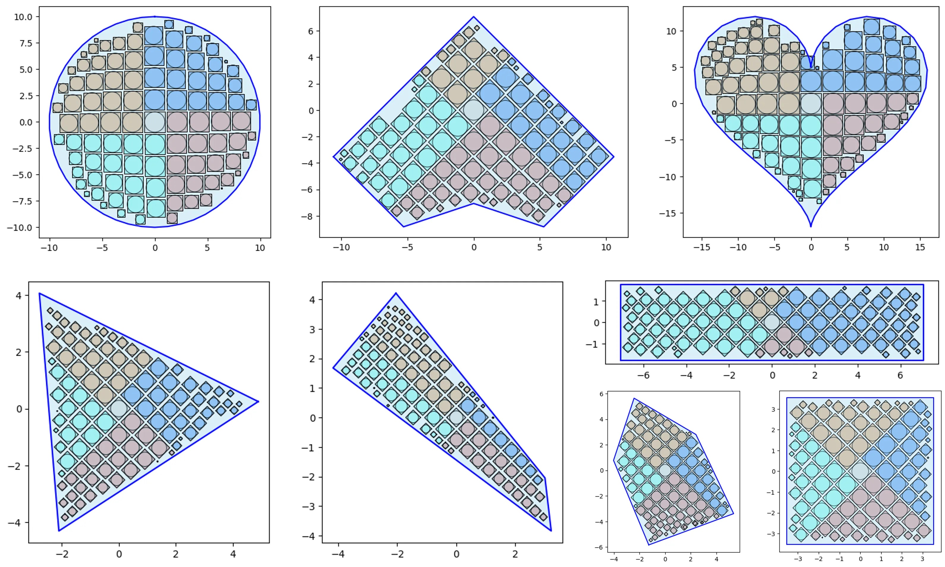
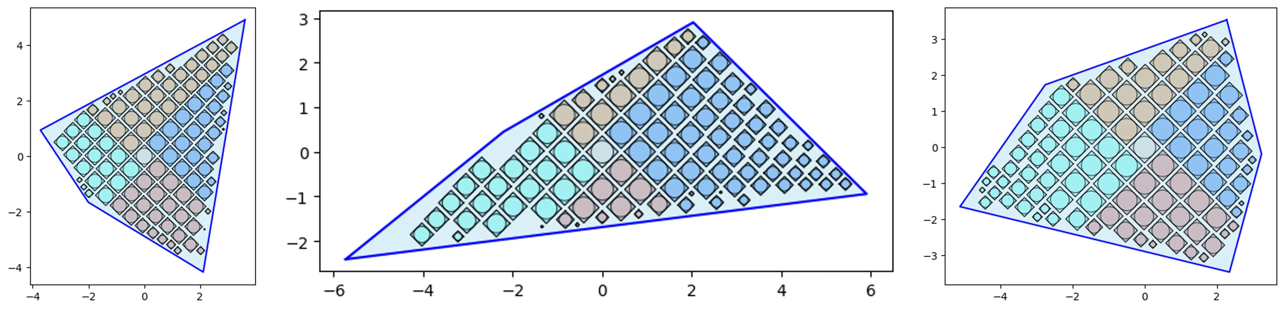
More complicated (random) containers examples:
pqt_o = pqt.random_polyquadtile(100, collapse=True)
pqt_o.polyquadtile_plot(color='quad', cw=0.75, opacity=.9, circles=True,
    show_constraints=True)

# keep executing for random containers with randomly sized squares
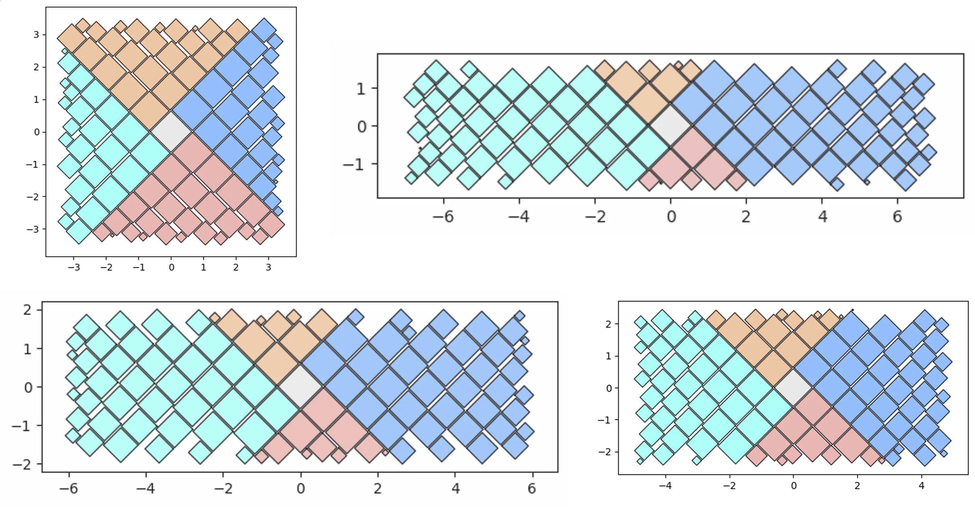
By aspect ratio:
aspect_ratio = (1,1) #(2,1) (3,1) (4,1)
pqt_o = pqt.random_polyquadtile(100, constraints=[aspect_ratio],
    rotate=45, collapse=True, buffer=.02)
pqt_o.polyquadtile_plot(color='quad', cw=0.75, opacity=.9)
Outputs:
from vizmath.quadtile_chart import polyquadtile as pqt
import pandas as pd
# using the initial example data with no resizing (fit's in container):
data = {
'id' : [str(i) for i in range(1, 21)],
'speed' : [242,200,105,100,100,95,92.5,88,80,79,
75,67.85,61.06,60,56,55,55,55,50,50]
}
poly = [(-1000,-1000),(-1000,1000),(1000,1000),
(1000,-1000)] # big enough container (for explaining example output)
df = pd.DataFrame(data)
o_pq1 = pqt(df,'id','speed',buffer=5.0, collapse=True,
constraints=poly, auto=False)
o_pq2 = pqt(df,'id','speed',buffer=5.0, collapse=True,
constraints=poly, auto=False, size_by='width')
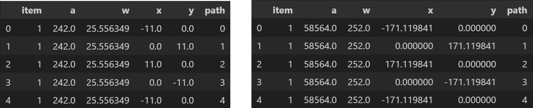
# size by area:
o_pq1.o_polyquadtile_chart.df[['id','item','a','w','x','y','path']].head()
# size by width:
o_pq2.o_polyquadtile_chart.df[['id','item','a','w','x','y','path']].head()
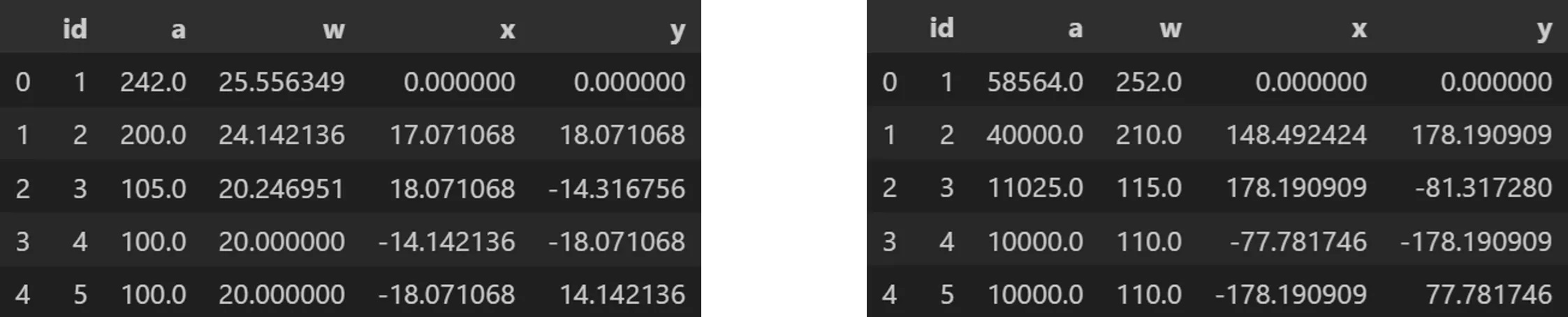
Centroids:
# size by area:
o_pq1.o_polysquares.df[['id','a','w','x','y']].head()
# size by width:
o_pq2.o_polysquares.df[['id','a','w','x','y']].head()
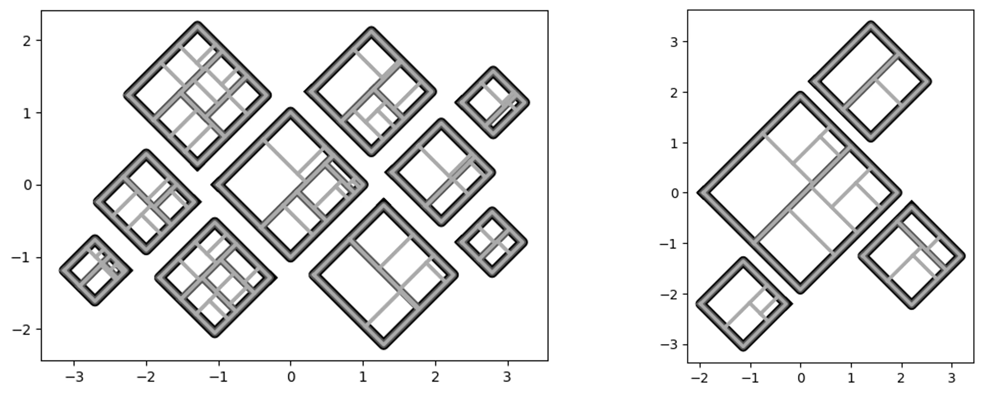
Squaremap
import pandas as pd
from vizmath.quadtile_chart import squaremap as sm

# generate a random square map
o_sm1 = sm.random_squaremap(num_levels=3, items_range=(2,4),
    value_range=(1,1000), sig=0.8)
o_sm1.o_squaremap.plot_levels(level=3, fill='w')

# create a square map from hierachical data
data = [
    ['a1', 'b1', 'c1', 9.3],
    ['a1', 'b1', 'c2', 6.7],
    ['a1', 'b1', 'c3', 2.4],
    ['a1', 'b2', 'c1', 4.5],
    ['a1', 'b2', 'c2', 3.1],

    ['a2', 'b1', 'c1', 5.9],
    ['a2', 'b1', 'c2', 32.3],
    ['a2', 'b1', 'c3', 12.3],
    ['a2', 'b1', 'c4', 2.3],
    ['a2', 'b2', 'c1', 9.1],
    ['a2', 'b2', 'c2', 17.3],
    ['a2', 'b2', 'c3', 6.7],
    ['a2', 'b2', 'c4', 4.4],
    ['a2', 'b2', 'c5', 11.3],

    ['a3', 'b1', 'c1', 7.5],
    ['a3', 'b1', 'c2', 9.5],
    ['a3', 'b2', 'c3', 17.1],

    ['a4', 'b2', 'c1', 5.1],
    ['a4', 'b2', 'c2', 2.1],
    ['a4', 'b2', 'c3', 11.1],
    ['a4', 'b2', 'c4', 1.5]]
df = pd.DataFrame(data, columns = ['a', 'b', 'c', 'value'])
o_sm2 = sm(df, ['a','b','c'], 'value', constraints=[(1,1)], buffer=.2)
o_sm2.o_squaremap.plot_levels(level=3, fill='w')
coming soon
Planning to retire the dataoutsider package and move over my multi-chord diagram to vizmath, with many more new algorithms to come! - as time permits :)
walkthroughs
Check out https://medium.com/@nickgerend for detailed tutorials and in-depth looks at the various method parameters (including Tableau Public tips!)
Release history Release notifications | RSS feed


Download files
Download the file for your platform. If you're not sure which to choose, learn more about installing packages.
Source Distribution
Built Distribution
Filter files by name, interpreter, ABI, and platform.
If you're not sure about the file name format, learn more about wheel file names.
Copy a direct link to the current filters
File details
Details for the file vizmath-0.0.47.tar.gz.
File metadata
- Download URL: vizmath-0.0.47.tar.gz
- Upload date:
- Size: 66.4 kB
- Tags: Source
- Uploaded using Trusted Publishing? No
- Uploaded via: twine/6.0.1 CPython/3.11.8
File hashes
| Algorithm | Hash digest | |
|---|---|---|
| SHA256 |
39720c6d14e67737b89b77cbda9d659bea3a84b352ecae85c5c433348912c863
|
|
| MD5 |
d16d68a85ed73a2d7d1480f0a68e1d47
|
|
| BLAKE2b-256 |
acdc112d54e698a60563a964de67571d98604239ad3c8a052640d9ef660d0e6f
|
File details
Details for the file vizmath-0.0.47-py3-none-any.whl.
File metadata
- Download URL: vizmath-0.0.47-py3-none-any.whl
- Upload date:
- Size: 54.4 kB
- Tags: Python 3
- Uploaded using Trusted Publishing? No
- Uploaded via: twine/6.0.1 CPython/3.11.8
File hashes
| Algorithm | Hash digest | |
|---|---|---|
| SHA256 |
fa7cb4d239c80a5bea3bb78f46b2e71034c5c05f18115afa7d255624cc1926c2
|
|
| MD5 |
c048f869bfe14ddb6b47d3e04f2dfd7d
|
|
| BLAKE2b-256 |
06968b12dbee42eff76e46b39c8c4157c79221df09903d60bf3c40ae86609c43
|


