
Python package for HLA imputation validation metrics using scikit-learn

Project description
VOIHLA - Validation of Imputed HLA
Compute high resolution HLA imputation validation metrics using the voihla Python package and scikit-learn model evaluation statistics.
Overview
The voihla package provides tools to preprocess, analyze, and visualize HLA imputation results. It supports single-locus, multilocus, and eplet-level analyses using standard metrics and calibration plots.
Installation
Install package and dependencies via pip:
pip install voihla
Example Input Files
imputation.csv: Imputation output with predicted HLA haplotype pairs and probabilities.truth_table.csv: High resolution genotype truth table in GLString format.
Example contents of files that are input for the package:
imputation.csv
ID,Rank,Hap1,Hap2,HapPair_Prob
D3505,1,A*30:02~B*14:02,A*32:01~B*39:10,0.3150459288416418
D3505,2,A*30:02~B*14:02,A*32:01~B*39:01,0.2673517305598033
D3505,3,A*30:02~B*39:10,A*32:01~B*14:02,0.09971243338882652
D3505,4,A*30:02~B*14:02,A*32:01~B*39:06,0.09552497014201682
D3505,5,A*30:01~B*14:02,A*32:01~B*39:10,0.0787155933156964
D3505,6,A*30:01~B*14:02,A*32:01~B*39:01,0.06679899077690125
D3505,7,A*30:01~B*39:10,A*32:01~B*14:02,0.02920649369703246
D3505,8,A*30:01~B*14:02,A*32:01~B*39:06,0.02386732857916924
D3505,9,A*30:02~B*14:02,A*32:01~B*39:24,0.009453181190469357
D3505,10,A*30:01~B*14:02,A*32:01~B*39:24,0.002361918368107546
D3505,11,A*30:02~B*39:01,A*32:01~B*14:02,0.002257484294942207
D13880,1,A*30:02~B*07:02,A*34:02~B*53:01,0.40269177048888066
D13880,2,A*30:01~B*07:02,A*34:02~B*53:01,0.20308144129546576
D13880,3,A*30:02~B*53:01,A*34:02~B*07:02,0.13918038201193
D13880,4,A*30:01~B*53:01,A*34:02~B*07:02,0.11366198792610206
D13880,5,A*30:02~B*07:05,A*34:02~B*53:01,0.04839353857099623
D13880,6,A*30:01~B*07:05,A*34:02~B*53:01,0.04136109507629823
D13880,7,A*30:02~B*53:01,A*34:02~B*07:09,0.011395011799743957
D13880,8,A*30:02~B*53:01,A*34:02~B*07:05,0.010829180412477053
D13880,9,A*30:01~B*53:01,A*34:02~B*07:09,0.009305763318635456
D13880,10,A*30:01~B*53:01,A*34:02~B*07:05,0.008843675778868338
D13880,11,A*30:04~B*53:01,A*34:02~B*07:02,0.0027297420425591353
truth_table.csv
ID,GLString
D3505,A*30:02+A*32:01^B*14:02+B*39:01
D13880,A*30:02+A*34:02+B*07:05+B*53:01
Usage
All main modules are in the voihla folder.
Preprocessing
Convert raw imputation files to analysis-ready format:
from voihla.preprocessing import ImputationPreprocessor

preprocessor = ImputationPreprocessor()
top_impute = preprocessor.process_files(['imputation.csv']) # Can pass multiple files in a list
top_impute.to_csv('lowres_topprob_impute.csv', index=False)
This will create a variable that will have every GLString in the imputation file ready for SLUG and MUG analyses depending on how many loci are avaialble in your file.
Single-Locus Analysis
import pandas as pd
from voihla.analysis import SingleLocusAnalysis
from voihla.preprocessing import ImputationPreprocessor

preprocessor = ImputationPreprocessor()
impute_df = preprocessor.process_files(['imputation.csv'])
truth_df = pd.read_csv('truth_table.csv')  # If your truth table is in a clean format then you just need to create a DataFrame
analysis = SingleLocusAnalysis(truth_df, impute_df)
results = analysis.get_results_df()
print(results)
The results DataFrame will contain the the variables required for Calibration plots.
y_true = if the imputation matches the truth table then 1, otherwise 0.
y_pred = the confidence of the imputation prediction being correct 1, otherwise 0 (threshold is 0.5 and can be changed).
y_prob = the actual probability of the imputation.
Multilocus Analysis
from voihla import ImputationPreprocessor, MultiLocusAnalysis
import pandas as pd

preprocessor = ImputationPreprocessor()
impute_df = preprocessor.process_files(['imputation.csv'])
truth_df = pd.read_csv('truth_table.csv')
analysis = MultiLocusAnalysis(truth_df, impute_df)
results = analysis.get_results_df()
print(results)
The results DataFrame will contain the the variables required for Calibration plots.
y_true = if the imputation matches the truth table then 1, otherwise 0.
y_pred = the confidence of the imputation prediction being correct 1, otherwise 0 (threshold is 0.5 and can be changed).
y_prob = the actual probability of the imputation.
Calibration Plots
Calibration plots can be generated using the CalibrationPlotter class from the voihla.plotting module. Below is an example calibration plot that can be generated by this module. This is using data found in a conference abstract.
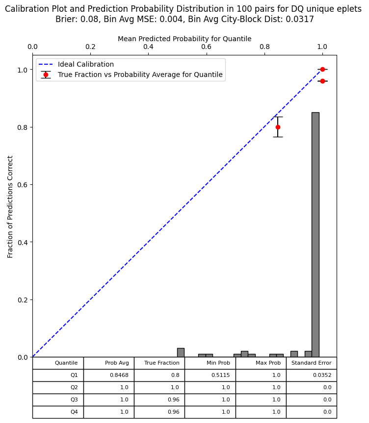
Can take either SingleLocusAnalysis or MultiLocusAnalysis results DataFrame as input.
from voihla.plotting import CalibrationPlotter

plotter = CalibrationPlotter(n_bins=4)
locus = 'A'
df = analysis.get_results_df()[locus]
fig = plotter.calibration_plot(analysis_results=df, title=f'Calibration {locus}', save_path=f'Calibration_{locus}.png')
Eplet-Level Analysis
Eplet analysis requires an API key from the EpRegistry if you do not already have the eplet mismatch lists. There are two classes: MonteCarloEpletAnalysis builds the input files by querying the EpRegistry API, and EpletAnalysis runs calibration analysis on the results.
Step 1 — Build truth and imputed eplet tables (MonteCarloEpletAnalysis)
MonteCarloEpletAnalysis takes a truth pairs file and an imputation pairs file and queries the EpRegistry API to produce eplet mismatch counts for both. The PairProb column in the imputed file comes from the product of the donor and recipient genotype frequencies in the imputation output (computed upstream by DRDQ_pair_simulation.py).
The which_impute argument controls which locus is analyzed: 'DRDQ', 'DR', or 'DQ'.
Required columns in the truth pairs file ({locus}_pairs_truth.csv):
DON_ID,REC_ID,DON_GLString,REC_GLString
Required columns in the imputation pairs file ({locus}_pairs_imputation.csv):
DON_ID,REC_ID,PairProb_{locus},DON_{locus},REC_{locus}
from voihla.eplet import MonteCarloEpletAnalysis

# Load API key from a local file (keep this out of version control)
mc = MonteCarloEpletAnalysis.from_key_file('api.key')

# Step 1 — sample n random pairs from the truth pairs file
truth_pairs = mc.sample_pairs(
    'DRDQ_pairs_truth.csv',
    n_pairs=100,
    save_path='DRDQ_pairs_truth_100.csv'
)

# Step 2 — query API with high-resolution truth genotypes -> truth eplet table
truth_eplets = mc.build_truth_eplet_table(
    truth_pairs,
    which_impute='DRDQ',
    save_path='DRDQ_eplet_truth_table100.csv'
)

# Step 3 — pull all imputation rows for those pairs out of the imputation file
impute_rows = mc.get_imputation_rows(
    'DRDQ_pairs_imputation.csv',
    truth_pairs,
    which_impute='DRDQ',
    save_path='DRDQ_pairs_imputation_100.csv'
)

# Step 4 — query API with low-resolution imputed genotypes -> imputed eplet table
impute_eplets = mc.build_impute_eplet_table(
    impute_rows,
    which_impute='DRDQ',
    save_path='DRDQ_eplet_lowres_impute100.csv'
)
The API key can also be passed directly as a string:
mc = MonteCarloEpletAnalysis(api_key='your-key-here')
Step 2 — Calibration analysis (EpletAnalysis)
EpletAnalysis takes the truth eplet table and the imputed eplet table produced above and generates calibration plots for each locus present in both files. The imputed file must have a PairProb_* column — probabilities are aggregated by summing PairProb across all rows that share the same predicted eplet count for a given pair.
from voihla.eplet import EpletAnalysis

ea = EpletAnalysis(
    truth_file='DRDQ_eplet_truth_table100.csv',
    impute_file='DRDQ_eplet_lowres_impute100.csv',
)

plots = ea.run_calibration_analysis(n_bins=10)
After calling run_calibration_analysis(), results are stored on the instance:
# Per-pair results: one row per donor-recipient pair
# Columns: ID, y_true, y_pred, y_prob
print(ea.pair_results['Total'])   # DRDQ combined
print(ea.pair_results['DR'])
print(ea.pair_results['DQ'])

# Summary metrics per locus
print(ea.summary_results['DR']['brier'])            # Brier score
print(ea.summary_results['DR']['roc_auc'])          # ROC-AUC
print(ea.summary_results['DR']['confusion_matrix']) # DataFrame: TN, FP, FN, TP
Save plots and results:
import pandas as pd

# Save calibration plots
for name, fig in plots.items():
    fig.savefig(f'{name}.png', bbox_inches='tight', dpi=150)

# Save per-pair results to CSV
for locus, df in ea.pair_results.items():
    df.to_csv(f'eplet_pair_results_{locus}.csv', index=False)

# Save summary metrics to CSV
summary_rows = []
for locus, metrics in ea.summary_results.items():
    row = {'locus': locus, 'brier': metrics['brier'], 'roc_auc': metrics['roc_auc']}
    row.update(metrics['confusion_matrix'].iloc[0].to_dict())
    summary_rows.append(row)
pd.DataFrame(summary_rows).to_csv('eplet_summary_results.csv', index=False)
y_true = 1 if the most probable predicted eplet count matches the true count, otherwise 0.
y_pred = 1 if the probability of the top predicted count is ≥ 0.9, otherwise 0.
y_prob = summed probability of the most probable predicted eplet count across all imputation samples for that pair.
Output
- Calibration plots saved as PNG files
- ROC curves saved as PNG files
- Classification reports
- Summary CSV files
API Reference
Please go to the Eplet Registry for an API key.


Download files
Download the file for your platform. If you're not sure which to choose, learn more about installing packages.
Source Distribution
Built Distribution
Filter files by name, interpreter, ABI, and platform.
If you're not sure about the file name format, learn more about wheel file names.
Copy a direct link to the current filters
File details
Details for the file voihla-0.1.3.tar.gz.
File metadata
- Download URL: voihla-0.1.3.tar.gz
- Upload date:
- Size: 20.9 kB
- Tags: Source
- Uploaded using Trusted Publishing? No
- Uploaded via: twine/6.1.0 CPython/3.13.12
File hashes
| Algorithm | Hash digest | |
|---|---|---|
| SHA256 |
8d69d82e56e7fd1d569aaef0047ad6f2af88861783e39c47b5ac7bdb93805345
|
|
| MD5 |
f1e5576512898406a30e6b5ad27e4562
|
|
| BLAKE2b-256 |
ca5db47f53bee301d6ae989956c541fddb2142ca8bc557b44e034af06e0674b3
|
File details
Details for the file voihla-0.1.3-py3-none-any.whl.
File metadata
- Download URL: voihla-0.1.3-py3-none-any.whl
- Upload date:
- Size: 19.5 kB
- Tags: Python 3
- Uploaded using Trusted Publishing? No
- Uploaded via: twine/6.1.0 CPython/3.13.12
File hashes
| Algorithm | Hash digest | |
|---|---|---|
| SHA256 |
35f10cbe42e2c5032b6ddae00e4afdd4ce7309818e36de184d0e959b1163520f
|
|
| MD5 |
705b5283690dbd39f3b40bd4aee3da28
|
|
| BLAKE2b-256 |
2e452c07aa7ca89204144ddf105185912809a674fa360c76e4d3b44f519f7ae1
|






