
volVIC — VOLume-based Virtual Image Correlation
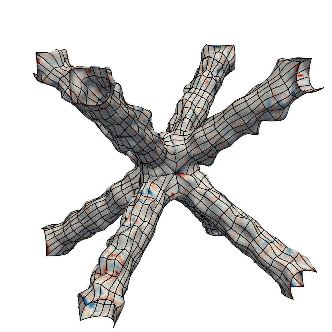
volVIC is a Python library for surface shape measurement from 3D volumetric images (e.g. CT scans) using the Virtual Image Correlation (VIC) method. It fits a parametric B-spline surface mesh to a grayscale volume by minimizing an energy functional that compares a synthetic "virtual image" — built from the surface geometry — to the actual acquired image.
The method is particularly suited to problems in experimental mechanics, where one wants to track the shape or deformation of a material surface from tomographic data.
Table of Contents
Method overview
The VIC approach replaces classical pixel-to-pixel image correlation with a physics-motivated model. Given a B-spline surface mesh and a volumetric image:
- A virtual image is constructed analytically from the surface geometry. It models the gray-level transition (background ↔ foreground) along the surface normal, parameterized by a scalar distance
rho. - The VIC energy measures the discrepancy between the virtual image and the actual acquired image, integrated over a normal neighborhood of the surface.
- A Gauss–Newton solver iteratively minimizes the total energy (VIC + membrane regularization) with respect to the B-spline control point displacements and
rho. - C¹ continuity constraints across patches and Dirichlet boundary conditions are enforced through a constraint matrix.
Installation
1. High-Performance Solvers (Optional but Recommended)
volVIC relies on IGA_for_bsplyne for its linear system solvers. This library can leverage SuiteSparse (via scikit-sparse and sparseqr) for significant speedups on large-scale problems.
-
Recommended (Conda):
conda install -c conda-forge scikit-sparse
pip install sparseqr
Note:
sparseqris not on Conda, but it will successfully link to the SuiteSparse libraries installed byscikit-sparse. -
Alternative (system package manager):
- macOS:
brew install suitesparse && pip install scikit-sparse sparseqr - Ubuntu/Debian:
sudo apt-get install libsuitesparse-dev && pip install scikit-sparse sparseqr
- macOS:
-
Fallback: If SuiteSparse is not available, the library automatically falls back to standard
scipy.sparsesolvers, ensuring full compatibility at the cost of performance.
2. Install volVIC
pip install volVIC
Requirements: Python ≥ 3.9
Key dependencies: numpy, scipy, numba, bsplyne, IGA_for_bsplyne, pyvista, meshio, interpylate, treeIDW, matplotlib, tqdm
Quick start
import numpy as np
from volVIC import Mesh, Problem

# Load your B-spline surface mesh and volumetric image
mesh = Mesh.Mesh.load("my_mesh.pkl")
image = np.load("my_ct_scan.npy")   # dtype: uint16, shape: (Z, Y, X)

# Set up and solve the VIC problem
problem = Problem(
    mesh=mesh,
    image=image,
    ICP_init=True,         # Rigid-body alignment before solving
    C1_mode="auto",        # Automatic C¹ continuity between patches
    membrane_weight=None,  # Automatic regularization weight estimation
)
u_field, rho = problem.solve(max_iter=20)

# Visualize results
problem.plot_results(u_field)

# Export to ParaView
problem.save_paraview(u_field, folder="results/", name="vic_output")
Module overview
volVIC.Problem — High-level solver
The main entry point. The Problem class encapsulates the full VIC pipeline.
Constructor Problem(mesh, image, ...):
- Estimates foreground/background gray levels from the image histogram (Otsu or interpolation-based).
- Optionally performs a rigid-body ICP alignment of the mesh to the image isosurface.
- Builds the virtual image energy elements, membrane stiffness matrix, and C¹ constraint matrix.
- Calibrates the membrane regularization weight automatically.
Key methods:
| Method | Description |
|---|---|
solve(max_iter, ...) |
Run the Gauss–Newton optimization loop. Returns (u_field, rho). |
plot_results(u_field, ...) |
Visualize signed distance fields with PyVista. |
save_paraview(u_field, folder, name) |
Export displacement and distance fields to VTK for ParaView. |
propagate_displacement_to_volume_mesh(u_field, volume_mesh) |
Propagate the surface displacement to a volumetric B-spline mesh. |
volVIC.Mesh — B-spline mesh management
Provides the Mesh class wrapping multi-patch B-spline surfaces.
Key features:
- Load/save mesh from
.pkl(pickle) files (Mesh.load,Mesh.save). - Evaluate the mesh geometry and fields at arbitrary parametric points.
- Convert fields between per-patch and unique-node representations.
- Extract border patches, mesh subsets, and orientation fields.
- Visualize with PyVista (
plot,plot_in_image,plot_orientation). - Export time series to ParaView with
save_paraview. - Register mesh to a target triangle surface with
ICP_rigid_body_transform. - Propagate scalar or vector fields from a submesh to a parent mesh.
volVIC.virtual_image_correlation_energy — VIC energy
The VirtualImageCorrelationEnergyElem class handles the energy computation for a single B-spline patch. It:
- Builds integration grids in both parametric and normal directions.
- Constructs the sparse small rotation displacement operator mapping control points to integration points in the image.
- Evaluates the VIC energy, gradient, and Gauss-Newton Hessian w.r.t. displacements and
rho.
The module also provides utilities:
make_image_energies(mesh, h, ...)— initialize energy elements for a full mesh.compute_image_energy_operators(...)— assemble global gradient and Hessian.compute_distance_field(...)— compute the signed distance field on each patch.
volVIC.virtual_image — Virtual image model
Defines the virtual image function used in the VIC energy:
from volVIC.virtual_image import g_slide

g, dg_drho = g_slide(xi, eta, gamma, rho, bg=0.0, fg=1.0)
g_slide models a smooth transition from background to foreground gray level along the surface normal (gamma), parameterized by the half-width rho. It returns both the image value g and its derivative w.r.t. rho.
volVIC.solve — Gauss–Newton iteration
Low-level function performing one VIC iteration:
from volVIC.solve import iteration

du_field, drho = iteration(u_field, rho, mesh, image_energies, image,
                           membrane_K, membrane_weight, C)
Assembles and solves the linearized system H_tot @ Δu = -grad_tot, with constraint enforcement via the matrix C. The rho increment is computed independently by a Newton step on the scalar energy.
volVIC.membrane_stiffness — Regularization
Assembles the membrane (in-plane) stiffness matrix for B-spline surface patches, used as a regularization term in the VIC energy:
from volVIC.membrane_stiffness import make_membrane_stifness, make_membrane_weight

K = make_membrane_stifness(mesh)
w = make_membrane_weight(mesh, image_energies, K, rho=1.5, image_std=5000)
The make_membrane_weight function calibrates the regularization weight by matching the expected membrane energy to the expected VIC energy under a probabilistic displacement model.
volVIC.C1_triplets — Smoothness constraints
Generates C¹ continuity constraints between neighboring patches:
from volVIC.C1_triplets import make_C1_eqs

C = make_C1_eqs(mesh, C1_inds="auto", threshold=0.1)
Each constraint takes the form A - 2B + C = 0 for a triplet of control nodes (A, B, C). The "auto" mode selects only geometrically consistent triplets.
volVIC.image_utils — Image preprocessing
Utilities for gray-level analysis of CT images:
from volVIC.image_utils import find_fg_bg, find_sigma_hat

fg, bg = find_fg_bg(image, method="otsu")   # or "interp"
sigma  = find_sigma_hat(image, fg, bg)
find_fg_bgestimates foreground and background gray levels from the image histogram.find_sigma_hatestimates the noise standard deviation from single-phase voxels.- Lower-level functions
hist,otsu_threshold, andinterp_fg_bgare also exposed.
volVIC.marching_cubes — Isosurface extraction
Extracts a triangle isosurface from a 3D scalar field:
from volVIC.marching_cubes import marching_cubes

surface = marching_cubes(volume, threshold=0.5)  # returns meshio.Mesh
Uses a Numba-compiled implementation for performance, with vertex deduplication and zero-area triangle prevention.
volVIC.integration_space_image — Parametric integration
Computes integration points and weights in the parametric space of a B-spline surface such that mapped distances between points are approximately uniform:
from volVIC.integration_space_image import linspace_for_VIC_elem

(xi, eta), (dxi, deta) = linspace_for_VIC_elem(spline, ctrl_pts, dist=1.0)
Documentation
The full API documentation is available on the Online Portal.
License
This project is licensed under the CeCILL-2.1 license — see https://cecill.info for details.
Author: Dorian Bichet — dbichet@insa-toulouse.fr
Repository: https://github.com/Dorian210/volVIC
1 maintainer

Metadata
1 maintainer
Release files for volVIC 1.0.2
For a detailed explanation of source distributions (sdists) and built distributions (wheels), please see the package formats documentation.
Source distribution (sdist)
| File | Size | Uploaded | |
|---|---|---|---|
| volvic-1.0.2.tar.gz | 66.2 kB | Details |
Built distribution (wheel)
| File | Interpreter | ABI | Platform | Reset |
|---|---|---|---|---|
| volvic-1.0.2-py3-none-any.whl | Python 3 | none | any | Details |
Total release size: 133.2 kB
Release files / volvic-1.0.2.tar.gz
| Download URL | volvic-1.0.2.tar.gz |
|---|---|
| Size | 66.2 kB |
| Tags | Source |
|
SHA-256 checksum How to use checksums |
aad038b3ef432fde09ecbf79e4c13db168c2dd76a831aa01fb76ffc42438285a
|
|
BLAKE2b-256 checksum How to use checksums |
44efde8a30ac2cc790aa78a35fe50880f5cc3dbcc4f6bf847043fc3087c2ff7f
|
| Upload date | |
|
Uploaded using Trusted Publishing? What is trusted publishing? |
No |
| Uploaded via |
twine/6.2.0 CPython/3.14.3
|
Release files / volvic-1.0.2-py3-none-any.whl
| Download URL | volvic-1.0.2-py3-none-any.whl |
|---|---|
| Size | 67.0 kB |
| Tags | Python 3 |
|
SHA-256 checksum How to use checksums |
4e722c9a8823a12e81f75645675d9f0896750a8782078e3f244bf08ae68e1427
|
|
BLAKE2b-256 checksum How to use checksums |
a59eac05bbd32740ea46eb099f765bbe4d5a11aa2192b17cbedbd01eae34b090
|
| Upload date | |
|
Uploaded using Trusted Publishing? What is trusted publishing? |
No |
| Uploaded via |
twine/6.2.0 CPython/3.14.3
|














