WARP-Q: Quality Prediction For Generative Neural Speech Codecs

Project description
WARP-Q: Speech Quality Prediction For Generative Neural Speech Codecs
A Python package for running WARP-Q, a speech quality prediction metric for generative neural speech codecs.
WARP-Q is a Python library designed to evaluate the quality of modern generative neural speech codecs and traditional low bit-rate speech coders. It uses a subsequence dynamic time warping (SDTW) algorithm to measure the similarity between a reference (original) and a test (degraded) speech signal, producing raw and normalized quality scores.
Full design and details of WARP-Q are presented in the following papers:
- W. A. Jassim, J. Skoglund, M. Chinen, and A. Hines, “Speech quality assessment with WARP‐Q: From similarity to subsequence dynamic time warp cost,” IET Signal Processing, 1–21 (2022).
- W. A. Jassim, J. Skoglund, M. Chinen, and A. Hines, “WARP-Q: Quality prediction for generative neural speech codecs,” ICASSP 2021 - IEEE International Conference on Acoustics, Speech, and Signal Processing, 2021, pp. 401–405.
Features
- Efficient Computation: Compute WARP-Q scores for individual audio files or batches of files from CSV inputs.
- Full Customization: Users can easily modify parameters to adjust time and frequency domain resolutions according to your specific needs.
- Flexible SDTW Parameters: The library allows for the customization of parameters related to Soft Dynamic Time Warping (SDTW), enhancing its adaptability for various applications.
- Alignment Indices: WARP-Q provides time and frame indices for aligned audio segments of reference and corresponding degraded speech, facilitating in-depth quality analysis.
- Score Normalization: Normalize WARP-Q scores to a standardized scale for consistent evaluation.
- Useful Utility Functions: Access utility functions for plotting WARP-Q results, aggregating data, and loading audio files.
- Detailed Results Management: Save the obtained detailed results in DataFrames for better analysis and investigations.
- Accelerated Processing: Leverage parallel processing to speed up WARP-Q score computations.
Installation
You can install WARP-Q directly from PyPI:
pip install warpq
Usage
1. Importing the Package
Once installed, you can import the WARP-Q metric class:
from warpq.core import warpqMetric
You can also import utility functions:
from warpq.utils import load_audio, plot_warpq_scores, group_dataframe_by_columns
To create an instance of the warpqMetric class and initialize the model with default parameters, we run:
# Create an instance of the warpqMetric class
model = warpqMetric()
Loading the warpqMetric object will create an instance of the class with the following parameters:
-
sr:int(default:16000): Sampling frequency of audio signals in Hertz (Hz). -
frame_ms:int(default:32): Length of audio frame in milliseconds for framing. -
overlap_ms:int(default:4): Length of overlap between consecutive frames in milliseconds. -
n_mfcc:int(default:13): Number of Mel-Frequency Cepstral Coefficients to compute. -
fmax:int(default:5000): Cutoff frequency for MFCC computation. -
patch_size:float(default:0.4): Size of each patch in seconds for processing. -
patch_hop:float(default:0.2): Hop size between patches in seconds. -
sigma:list(default:[[1, 0], [0, 3], [1, 3]]): Step size conditions for Subsequence Dynamic Time Warping (SDTW). -
apply_vad:bool(default:True): Flag to determine if Voice Activity Detection (VAD) should be applied. -
score_fn:str(default:'median'): Function to compute the final score. Options are'mean'or'median'. -
cmvnw_win_time:float(default:0.836): The size of the sliding window for local normalization (in seconds). -
max_score:float(default:3.5): Maximum raw score for normalization. -
n_jobs:int(default:-1): Number of cores to use for parallel processing. IfNoneor-1, all available cores will be used.
We can also call the warpqMetric class with customized parameters. For example:
# Initialize the class with custom parameters
model = warpqMetric(sr=8000, frame_ms=25, overlap_ms=10)
This allows you to set custom values for parameters such as the sampling rate (sr), frame length (frame_ms), and overlap between frames (overlap_ms), among others.
2. Evaluating Quality of Two Audio Files
The evaluate() function from the warpqMetric class computes the WARP-Q score between two input speech signals, which can either be audio file paths or audio arrays. This function provides detailed alignment information, including the degree of similarity between the reference and degraded audio using the WARP-Q metric.
Inputs:
ref_audio: Path to the reference audio file or a NumPy array of the reference audio signal.deg_audio: Path to the degraded audio file or a NumPy array of the degraded audio signal.arr_sr: Sampling rate, required only if providing audio arrays.save_csv_path: Path to save the detailed results in a CSV file. IfNone, results are not saved. If a valid path is provided, the results will be saved in CSV format, with columns including reference and degraded audio descriptions, WARP-Q scores, alignment costs, and timing information for each patch. If the file already exists, new results will be appended without the header.verbose: IfTrue, outputs messages about the processing.
Outputs:
The evaluate() function returns a dictionary containing the WARP-Q results and detailed alignment information, including:
-
raw_warpq_score: The computed WARP-Q score between the reference and degraded audio. -
normalized_warpq_score: The normalized WARP-Q score between0and1, where1indicates the best audio quality. Please see the normalization section below for more details. -
total_patch_count: The total number of patches generated from the degraded signal's MFCC, representing the number of segments in the degraded signal after applying the sliding window. -
alignment_costs: A list of DTW alignment costs for each degraded MFCC patch, representing how well each patch matches its aligned subsequence in the reference MFCC. Length is equal tototal_patch_count. -
aligned_ref_time_ranges: List of (start_time, end_time) tuples containing the start and end time stamps (in seconds) for the best matching subsequences in the reference MFCC, as aligned to each patch in the degraded signal using DTW. Length is equal tototal_patch_count. -
aligned_ref_frame_indices: List of (a_ast,b_ast) tuples containing the start and end frame indices for the best matching subsequences in the reference MFCC, corresponding to the aligned subsequences. Length is equal tototal_patch_count. -
deg_patch_time_ranges: List of (start_time, end_time) tuples containing the start and end time stamps (in seconds) for each patch in the degraded signal's MFCC, generated using a sliding window approach. Length is equal tototal_patch_count. -
deg_patch_frame_indices: List of (start_frame, end_frame) tuples containing the start and end frame indices for each patch in the degraded signal's MFCC, corresponding to the patches created by the sliding window process. Length is equal tototal_patch_count.
Example Usage:
You can compute the WARP-Q score between two audio files (reference and degraded) as follows:
# Create an instance of the warpqMetric class
model = warpqMetric()

# Evaluate the audio quality between two files
results = model.evaluate('audio/ref_audio.wav', 'audio/deg_audio.wav', verbose=True)

# Access the raw WARP-Q and normalized scores
raw_warpq_score = results["raw_warpq_score"]
normalized_warpq_score = results["normalized_warpq_score"]

# Print the results
print(f"Raw WARP-Q Score: {raw_warpq_score}")
print(f"Normalized WARP-Q Score: {normalized_warpq_score}")
3. Save detailed results to a CSV file
It is possible to save the results obtained from the model.evaluate function to a CSV file for further analysis. This can be done by setting the parameter save_csv_path to the desired file path:
results = model.evaluate('audio/ref_audio.wav', 'audio/deg_audio.wav', save_csv_path="csv/results.csv", verbose=True)
Below is an example of a few rows from the saved CSV file:

4. Evaluate Two Audio Arrays
You can load audio files using the load_audio function and pass the audio data to the model.evaluation function as shown in the following example:
# Load the reference and degraded audio files
ref_arr, deg_arr, ref_sr, deg_sr = load_audio(ref_path="audio/ref_audio.wav", deg_path="audio/deg_audio.wav", sr=16000, native_sr=False, verbose=True)

# Run the model using the loaded audio arrays
results = model.evaluate(ref_arr, deg_arr, arr_sr=ref_sr)
Note that the value passed to the arr_sr parameter should match the class-defined sampling rate self.sr.
5. Evaluate Batches of Files From CSV Inputs
The evaluate_from_csv from the warpqMetric class allows you to compute the WARP-Q scores for multiple audio files listed in a CSV file. This is useful when you need to evaluate the quality of audio for a large number of file pairs (reference and degraded).
The evaluate_from_csv function takes the following inputs:
input_csv(str): Path to a CSV file with specified reference and degraded wave columns.ref_wave_col(str): Name of the reference wave column. Default is'ref_wave'.deg_wave_col(str): Name of the degraded wave column. Default is'deg_wave'.raw_score_col(str): Column name where raw scores will be saved. Default is'Raw WARP-Q Score'.output_csv(str): Path to save results. IfNone, results are not saved.save_details(bool): IfTrue, save detailed results (alignment costs, times) in the same DataFrame.
and it returns the following:
-
pd.DataFrame: DataFrame with computed WARP-Q scores and detailed results if requested. -
Additional detailed results (saved when
save_details=True) include:total_patch_count(int): The total number of patches in the degraded signal.alignment_costs(list): The alignment costs for each patch between the degraded and reference signals.deg_patch_time_ranges(list): List of tuples for (start, end) times in seconds of each patch in the degraded signal.aligned_ref_time_ranges(list): List of tupes for (start, end) times in seconds of the aligned segments in the reference signal.
Preparing the Input CSV File:
To use this function, first, you need to prepare a CSV file with columns specifying the reference and degraded audio files. The CSV file must contain at least the following two columns:
ref_wave: Column containing paths to the reference audio files.deg_wave: Column containing paths to the degraded audio files.
You may optionally include additional columns, such as Mean Opinion Score (MOS), degradation type, condition (experiment), and database for each file, if such information is accessible. These columns can facilitate further analysis, such as plotting WARP-Q scores against MOS or evaluating performance based on degradation types or experimental conditions.
An example of the CSV file:
| database | ref_wave | deg_wave | condition | degradation_type | MOS |
|---|---|---|---|---|---|
| set1 | ref_audio_1.wav | deg_audio_1.wav | condA | noise | 4.5 |
| set2 | ref_audio_2.wav | deg_audio_2.wav | condB | reverb | 3.8 |
| set3 | ref_audio_3.wav | deg_audio_3.wav | condC | echo | 4.1 |
| set4 | ref_audio_4.wav | deg_audio_4.wav | condD | clipping | 4.3 |
You can optionally add more columns, but the function will primarily rely on the ref_wave and deg_wave columns for evaluating the audio quality.
Example Usage
results_df = model.evaluate_from_csv(
            input_csv="audio_files.csv",
            ref_wave_col="ref_wave",
            deg_wave_col="deg_wave",
            raw_score_col="WARP-Q score",
            output_csv="results_df.csv",
            save_details=True
            )
Note that audio files with short durations are skipped in the computation, and their results are replaced with np.nan. Below is an example of how the results from the evaluate_from_csv function might look when saved to a CSV file.

The alignment_costs, deg_patch_time_ranges, and aligned_ref_time_ranges lists are saved as strings in the CSV file. To convert these strings back to Python lists, you can use ast.literal_eval:
import ast
import pandas as pd
import numpy as np

# Load the CSV file
df_loaded = pd.read_csv('results_df.csv')

# Convert the string back to lists, handling NaN values
df_loaded['alignment_costs'] = df_loaded['alignment_costs'].apply(lambda x: ast.literal_eval(x) if pd.notna(x) else np.nan)

print(df_loaded)
6. Visualizing WARP-Q Scores Using the plot_warpq_scores Function
The plot_warpq_scores function generates a scatter plot of MOS versus WARP-Q scores and calculates the Pearson and Spearman correlation coefficients. The function supports color encoding and marker styling based on categories such as condition or degradation_type to enhance the plot's clarity.
Parameters:
df: ApandasDataFrame or path to a CSV file containing MOS and WARP-Q scores.mos_col: The column name for theMOS.warpq_col: The column name for WARP-Q scores. Default is"Raw WARP-Q Score".hue_col: Optional. A column name used to color the points by category (e.g.,cnditionordegradation_type).style_col: Optional. A column name to differentiate marker styles in the scatter plot.save_path: Optional. The path to save the plot as a.pngfile. The.pngextension will be added if not provided.
By default, the function plots MOS and WARP-Q scores for each audio file in the dataset, allowing you to directly assess the relationship between subjective and objective quality metrics.
Example Usage (Plotting for Individual Files):
warp_plot = model.plot_warpq_scores(
    df="results_df.csv",          # Path to CSV containing MOS and WARP-Q scores for each audio file (e.g., obtained from the model.evaluate_from_csv function)
    mos_col="MOS",                # Column containing MOS
    warpq_col="WARP-Q score", # Column containing WARP-Q scores
    # warpq_col="Normalized WARP-Q score", # or plot the normalized quality scores
    title="MOS vs WARP-Q for Individual Files",
    save_path="mos_vs_warpq_individual.png"
)
This example generates a scatter plot comparing MOS and WARP-Q scores for each individual audio file. The plot is saved as mos_vs_warpq_individual.png.
7. Plotting Scores Grouped by Condition or Degradation Type
In addition to plotting scores for individual files, it is often insightful to group the data by specific conditions such as degradation type, experiment condition, database or codec. Grouping scores can help you better understand how different types of degradation impact audio quality and assess the overall performance of a codec or processing technique across multiple conditions.
To achieve this, you can first group the data using the group_dataframe_by_columns function, and then plot the aggregated results.
Parameters:
data: ApandasDataFrame to group. If not provided, data can be loaded from a CSV viacsv_path.csv_path: Path to a CSV file to load data from if no DataFrame is provided.group_cols: A list of columns to group by (e.g.,["Degradation Type", "Condition"]).agg_cols: A list of columns to apply the aggregation function to (e.g.,["MOS", "Raw WARP-Q Score"]).agg_func: The aggregation function to apply. Default is"mean", but you can also apply other functions like"sum","min","max", etc..output_csv: Optional. Path to save the grouped data as a CSV file.
Example Usage (Grouping Data by Degradation Type and Plotting):
# Group data by Degradation Type and calculate the mean MOS and WARP-Q scores for each group
grouped_df = model.group_dataframe_by_columns(
    csv_path="results_df.csv",        # Path to the CSV file
    group_cols=["degradation_type"],  # Grouping by degradation type
    agg_cols=["MOS", "WARP-Q score", 'Normalized WARP-Q score'],  # Columns to aggregate
    agg_func="mean",                  # Aggregating by mean values
    output_csv="grouped_by_degradation.csv"  # Save grouped data to a new CSV
)

# Plot the grouped data
warp_plot = model.plot_warpq_scores(
    df="grouped_by_degradation.csv",  # Use the grouped data
    mos_col="MOS",                    # Column containing aggregated MOS
    warpq_col="WARP-Q score",     # Column containing aggregated WARP-Q scores
    # warpq_col="Normalized WARP-Q score", # or plot the normalized quality scores
    hue_col="degradation_type",       # Color points by degradation type
    title="MOS vs WARP-Q by Degradation Type",
    #title="MOS vs normalized WARP-Q by Degradation Type",
    save_path="mos_vs_warpq_degradation.png"
)
8. WARP-Q Score Normalization
The WARP-Q metric provides raw scores that exhibit a negative correlation with quality. This means that lower values (closer to zero) indicate higher quality, while higher scores reflect lower quality. This behavior arises because WARP-Q is based on the alignment cost between the reference and degraded speech signals.
Why Alignment Cost Gives Negative Quality Score Correlation?:
The alignment cost is calculated using Subsequence Dynamic Time Warping (SDTW), which measures how well the degraded speech aligns with the reference speech over time. When the alignment cost is low, it indicates that the codec or degradation type has preserved the speech signal well, resulting in higher quality. Conversely, a high alignment cost suggests more distortion, meaning the signal quality has deteriorated.
Normalization Process:
To present WARP-Q scores with positive correlation (where higher scores indicate better quality), we normalize the raw WARP-Q scores to a 0 to 1 scale. The normalization is performed using the following equation:
$$ \text{Normalized WARP-Q Score} = 1 - \left(\frac{\text{Raw WARP-Q Score}}{\text{Max WARP-Q Score}}\right), $$ where:
- Raw WARP-Q Score is the score produced by the WARP-Q metric (based on subsequence DTW alignment cost).
- Max WARP-Q Score is a predefined maximum score used for normalization.
The Max WARP-Q Score is set to 3.5 based on evaluations across four different databases that are used in our papers. This value ensures that the normalized scores range from 0 to 1 with positive correlation to quality.
Handling Scores That Exceed the Max Score:
If the Max WARP-Q Score is set too low, the normalization term $\left(\frac{\text{Raw WARP-Q Score}}{\text{Max WARP-Q Score}}\right)$ can result in values greater than 1. In such cases, the normalized score $\left(1 - \left(\frac{\text{Raw WARP-Q Score}}{\text{Max WARP-Q Score}}\right)\right)$ becomes less than zero. To prevent this, the WARP-Q implementation clips all negative scores to 0.
Therefore, if you notice many scores are zero, this likely indicates that the Max WARP-Q Score is too low for your dataset or codec, and you may need to adjust it.
Adjusting the Max Score:
You can adjust the Max WARP-Q Score to better fit your specific use case or database. To do this, pass the desired maximum value when creating an instance of the WARP-Q class:
model = warpqMetric(max_score=your_desired_max_score)
This allows you to fine-tune the normalization process according to the characteristics of your dataset and codec performance, ensuring better alignment with subjective quality assessments.
Normalizing to a 1-to-5 Scale:
It is possible to normalize the raw WARP-Q score to align with the Mean Opinion Score (MOS), which typically ranges from 1 to 5. The normalization for this would be:
$$ \text{Normalized WARP-Q Score} (1-5) = 1 + 4 \times \left(1 - \frac{\text{Raw WARP-Q Score}}{\text{Max WARP-Q Score}}\right), $$
where:
- A score of 1 indicates low quality,
- A score of 5 indicates high quality.
In the current implementation, we are scaling the scores to the 0 to 1 range to keep things simple. A more robust mapping model based on machine learning algorithms is under development. It will be released soon and will provide better correlations with the subjective quality scores. Such a model can handle various distortion and coding scenarios more effectively.
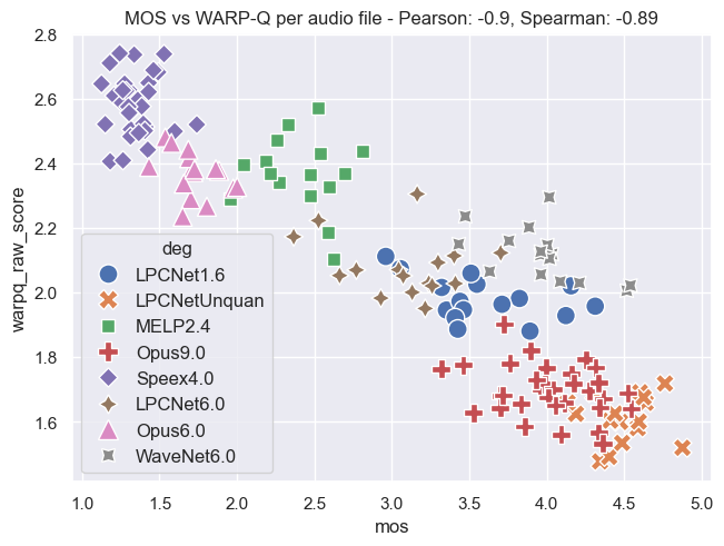
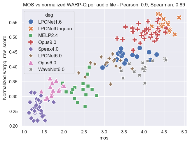
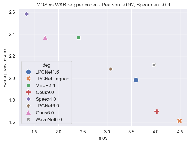
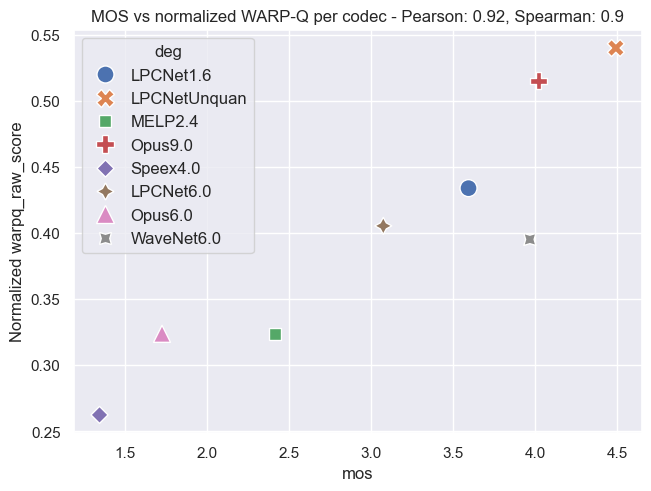
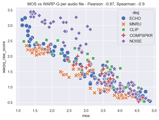
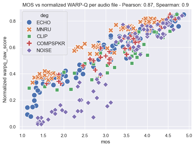
Plot Examples: MOS vs. WARP-Q Scores
The following plots demonstrate the relationship between MOS and WARP-Q scores, both before and after normalization. In the normalized plots, the WARP-Q scores are scaled from 0 to 1. These examples cover two cases:
- Per Audio File: This shows the alignment between MOS and WARP-Q scores for individual audio files.
- Per Codec: This demonstrates the comparison between MOS and WARP-Q scores aggregated by codec.
The plots are based on the Genspeech and TCD-VoIP databases described in the papers above and illustrate how normalization impacts score distribution and alignment between MOS and WARP-Q.
Genspeech Database
Per Audio File:
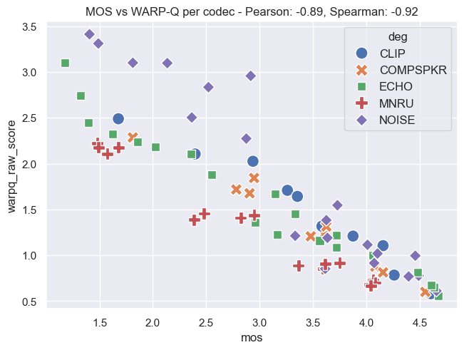
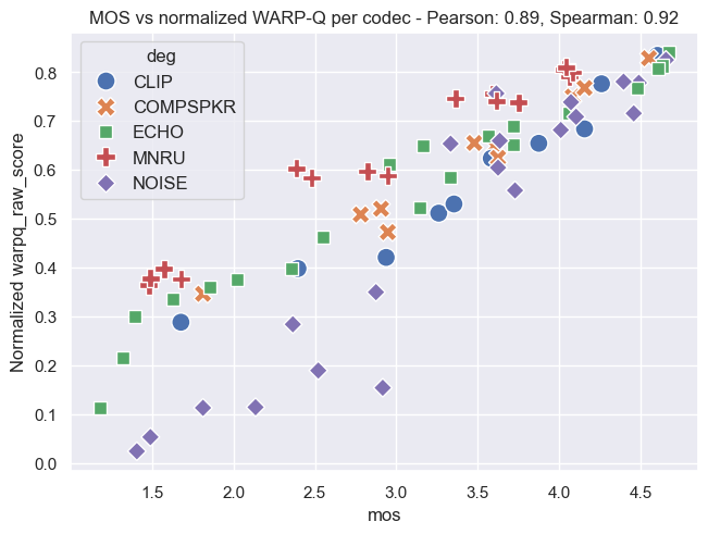
Per Codec:
TCD-VoIP Database
Per Audio File:
Per Codec:
Author
Dr Wissam A Jassim
wissam.a.jassim@gmail.com
October 6, 2024
Release history Release notifications | RSS feed


Download files
Download the file for your platform. If you're not sure which to choose, learn more about installing packages.
Source Distribution
Built Distribution
Filter files by name, interpreter, ABI, and platform.
If you're not sure about the file name format, learn more about wheel file names.
Copy a direct link to the current filters
File details
Details for the file warpq-1.5.2.tar.gz.
File metadata
- Download URL: warpq-1.5.2.tar.gz
- Upload date:
- Size: 50.6 kB
- Tags: Source
- Uploaded using Trusted Publishing? No
- Uploaded via: twine/5.1.1 CPython/3.10.14
File hashes
| Algorithm | Hash digest | |
|---|---|---|
| SHA256 |
659cc23b3d1d899f63f1096eb32e588dd353eecc76ef3e6c9416774ecf7a2690
|
|
| MD5 |
b61687a73170092728b48783c4bce623
|
|
| BLAKE2b-256 |
54558fba50b8bc462cf0e9b345132aa99d0bb0a595a3d6e43467c18edcabcdf4
|
File details
Details for the file warpq-1.5.2-py3-none-any.whl.
File metadata
- Download URL: warpq-1.5.2-py3-none-any.whl
- Upload date:
- Size: 28.9 kB
- Tags: Python 3
- Uploaded using Trusted Publishing? No
- Uploaded via: twine/5.1.1 CPython/3.10.14
File hashes
| Algorithm | Hash digest | |
|---|---|---|
| SHA256 |
e18781dfeff6568996d88ee6839083b53c63213cda5dd83504ca9f5f92c548b5
|
|
| MD5 |
31f9822fec22456ea3d3ffa2ca4e3db9
|
|
| BLAKE2b-256 |
6e387df0ec3ca6449c73adb758c6390c7e9c2d9887a5f551b87a0e6aa1a4887b
|


