WAve and WInd response prediction

Project description

What is WAWI?
WAWI is a Python toolbox for prediction of response of structures exposed to wind and wave excitation, using a multimodal frequency-domain approach. It supports special features such as:
- Hydrodynamic added mass, radiation damping and hydrodynamic force transfer function from e.g. WAMIT analysis
- Quasisteady wind forcing for buffeting analysis
- Combined effects of wind and waves
- Iterative multimodal flutter
- Iterative modal analysis
- Modelling of motion-induced aerodynamic forces using aerodynamic derivatives
- Inhomogeneous sea states
- Inhomogeneous mean wind (other parameters planned for)
- Current effects on wave excitation
- Stochastic linearization methodology to support linearized effect of quadratic drag damping (both line elements and pontoon objects)
- Object-oriented model setup, including FE description (using Python package BEEF) of beams exposed to aerodynamic forcing
Planned implemented in the near future:
- Fully inhomogeneous wind state definition (all wind field parameters)
- Hydrodynamic interaction effects from multibody analyses
- Second-order wave excitation effects
- Definition of ADs (aerodynamic derivatives) using rational functions
The package is still under development in its alpha stage, and documentation and testing will be completed along the way.
Installation
Either install via PyPI as follows:
pip install wawi
or install directly from github:
pip install git+https://www.github.com/knutankv/wawi.git@main
How does WAWI work?
By representing both aerodynamic and hydrodynamic motion-induced forces and excitation using a coordinate basis defined by the dry in-vacuum mode shapes of the structure, WAWI is able to versatily predict response based on input from any commercial FE software. The main structure used for response prediction is given in this figure:

The object structure of a WAWI model is given here:

Further details regarding hydrodynamic definitions initiated by the Hydro class is given below:

Further details regarding aerodynamic definitions initiated by the Aero class is given below:

Wave conditions
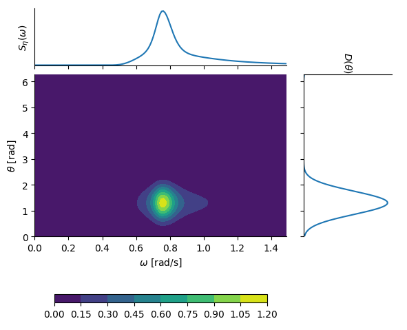
The wave field definition is based on the assumption that the two-dimensional wave spectral density can be decomposed into a directional distribution and a one-dimensional wave spectral density, i.e., $S_\eta(\omega,\theta) = D(\theta) S(\omega)$. The two factors are defined using these well-known formulations:
- $S(\omega)$: JONSWAP spectrum (see Hasselmann et al., 1973)
- $D(\theta)$: cos-2s directional distribution (see Longuet-Higgins et al., 1963)
Currents are defined by a homogeneous current speed U and corresponding direction thetaU.
An example of a two-dimensional wave spectral density based on (arbitrarily chosen) parameters $H_s = 2.1$ m, $T_p = 2.1$ s, $\gamma = 4.0$, $s = 10$ and $\theta_0 = 75^\circ$ is shown in this plot:
It is noted that you can easily assign custom functions of the S and D of the seastate (or customly on all pontoons for full control) instead of relying on the built in JONSWAP and cos-2s definitions.
Furthermore, as described in relevant examples, all sea state parameters can be defined as functions of x and y, to accomodate inhomogeneous sea states. In Kvåle et al. (2024), the effects of inhomogeneous sea states were analysed and were shown to be large for swell sea states with spherical wave fronts as illustrated here:

Wind conditions
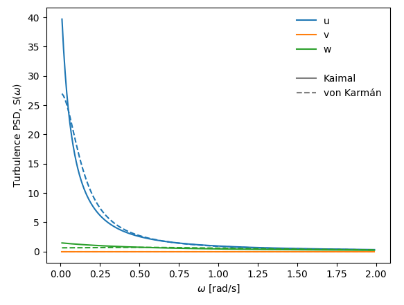
The wind field is defined by single-point turbulence wind spectra (for all turbulence components $u$, $v$ and $w$) and coherence definitions.
By default, wind spectra can be defined using these two definitions:
- Kaimal spectrum defined by length scale parameters ($L^x_u$, $L^x_v$, $L^x_w$), spectral shape parameters ($A_u$, $A_v$ and $A_w$) and turbulence intensities ($I_u$, $I_v$ and $I_w$); see Kaimal et al., 1972
- von Karmán spectrum defined by only length scale parameters ($L^x_u$, $L^x_v$, $L^x_w$) and turbulence intensities ($I_u=\sigma_u/U$, $I_v=\sigma_v/U$ and $I_w=\sigma_w/U$); see von Kármán, 1948
Furthermore, the coherence of the wind field is defined by the nine decay parameters $C_{ux}$, $C_{vx}$, $C_{wx}$, $C_{uy}$, $C_{vy}$, $C_{wy}$, $C_{uz}$ $C_{vz}$, $C_{wz}$; see e.g. Simiu and Scanlan, 1996 for details.
An example of turbulence spectral densities based on (arbitrarily chosen) parameters $I_u=0.136$, $I_v=0.0$, $I_w=0.072$, $L^x_u=115$, $L^x_w=9.58$, $A_u=6.8$ (only relevant for Kaimal-type) and $A_w=9.4$ (only relevant for Kaimal-type) is given below:
Quick start
Assuming a premade WAWI-model is created and saved as `MyModel.wwi´, it can be imported as follows:
from wawi.model import Model, Windstate, Seastate

model = Model.load('MyModel.wwi')
model.n_modes = 50                  # number of dry modes to use for computation
omega = np.arange(0.001, 2, 0.01)   # frequency axis to use for FRF
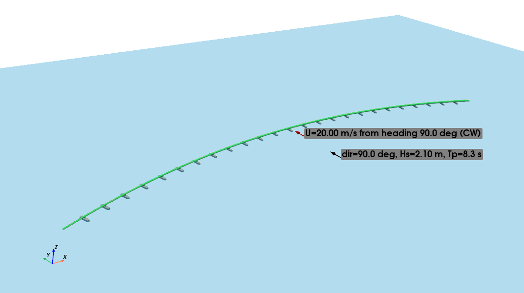
A windstate (U=20 m/s with origin 90 degrees and other required properties) and a seastate (Hs=2.1m, Tp=8.3s, gamma=8, s=12, heading 90 deg) is created and assigned to the model:
# Wind state
U0 = 20.0
direction = 90.0
windstate = Windstate(U0, direction, Iu=0.136, Iw=0.072,
                      Au=6.8, Aw=9.4, Cuy=10.0, Cwy=6.5,
                      Lux=115, Lwx=9.58, spectrum_type='kaimal')
model.assign_windstate(windstate)

# Sea state
Hs = 2.1
Tp = 8.3
gamma = 8
s = 12
theta0 = 90.0
seastate = Seastate(Tp, Hs, gamma, theta0, s)
model.assign_seastate(seastate)
The model is plotted by envoking this command:
model.plot()
which gives this plot of the model and the wind and wave states:
Then, response predictions can be run by the run_freqsim method or iterative modal analysis (combined system) conducted by run_eig:
model.run_eig(include=['hydro', 'aero'])
model.run_freqsim(omega)
The results are stored in model.results, and consists of modal representation of the response (easily converted to relevant physical counterparts using built-in methods) or modal parameters of the combined system (natural frequencies, damping ratio, mode shapes).
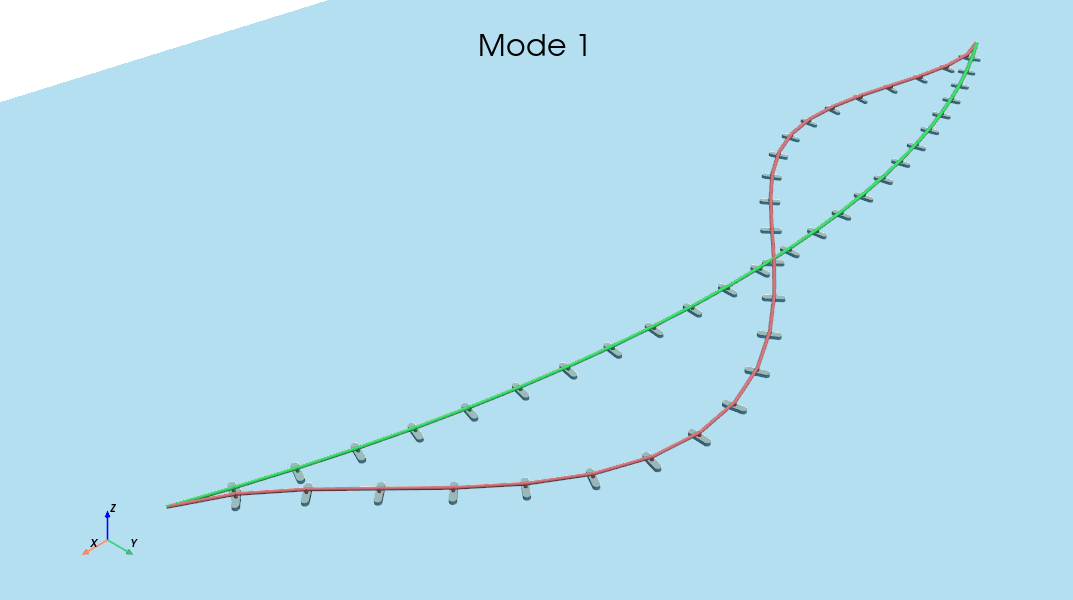
The resulting first mode shape is plotted as follows:
model.plot_mode(0)
This results in this plot:
For more details and recommendations regarding the analysis setup, it is referred to the examples provided and the code reference.
Examples
Examples are provided as Jupyter Notebooks in the examples folder.
The examples are structured in the following folders based on their topic:
- 0 Model generation and setup - Describing how a model is defined, either using input files together with the function
wawi.io.import_folderor using the classes available in thewawi.modelmodule directly (in the latter case, the open source Python library BEEF is used to create the required parameters directly in the notebook). - 1 Modal analysis - Describing how to set up iterative (and incremental) modal analyses to represent the contributions from aerodynamics and hydrodynamices. Also, an example showing how to set up a multi-modal flutter analysis is given.
- 2 Response prediction - Describing how to conduct response analyses using WAWI. This includes assigning wind states, sea states, and the necessary commands to run a frequency domain analysis. Furthermore, more advanced topics such as wave-current interaction, inhomogeneous waves and stochastic linearization to represent quadratic drag damping are given in separate examples. Three models are considered: (i) a simple curved floating bridge, (ii) a single beam, (iii) a suspension bridge.
- 3 Software interfacing - Describing how to export necessary data from other software (limited to Abaqus for now) to construct a WAWI model.
References
The following papers provide background for the implementation:
- Wave modelling and response prediction: Kvåle et al. (2016)
- Inhomogeneous wave modelling: Kvåle et al. (2024)
- Hydrodynamic interaction effects: Fenerci et al. (2022)
- Beam (FE) description of aerodynamic forces: Øiseth et al. (2012)
- Wave-current interaction: Fredriksen et al. (2024)
Citation
Please cite the use of this software as follows:
Kvåle, K. A., Fenerci, A., Petersen, Ø. W., & Øiseth, O. A. (2025). WAWI. Zenodo. https://doi.org/10.5281/zenodo.14895014

Support
Please open an issue for support.
Release history Release notifications | RSS feed


Download files
Download the file for your platform. If you're not sure which to choose, learn more about installing packages.
Source Distribution
Built Distribution
Filter files by name, interpreter, ABI, and platform.
If you're not sure about the file name format, learn more about wheel file names.
Copy a direct link to the current filters
File details
Details for the file wawi-0.0.19.tar.gz.
File metadata
- Download URL: wawi-0.0.19.tar.gz
- Upload date:
- Size: 108.3 kB
- Tags: Source
- Uploaded using Trusted Publishing? No
- Uploaded via: twine/6.1.0 CPython/3.9.22
File hashes
| Algorithm | Hash digest | |
|---|---|---|
| SHA256 |
268698b4ba3a3231567fde180122373acbc5b98f1b75bb9863ef9da5f7c9e285
|
|
| MD5 |
eb92c95043fb36ea0aed8c792c918329
|
|
| BLAKE2b-256 |
e5ca9892fc61fb4124b06893e63803d1332ac347159cec4a55f6dd470fd5e320
|
File details
Details for the file wawi-0.0.19-py3-none-any.whl.
File metadata
- Download URL: wawi-0.0.19-py3-none-any.whl
- Upload date:
- Size: 116.5 kB
- Tags: Python 3
- Uploaded using Trusted Publishing? No
- Uploaded via: twine/6.1.0 CPython/3.9.22
File hashes
| Algorithm | Hash digest | |
|---|---|---|
| SHA256 |
2b544502a4210c8b4b27eba20b30624fc24c8442be3edcaf356592d4e4297e15
|
|
| MD5 |
13d6c9a66032e67e24934072e98ce114
|
|
| BLAKE2b-256 |
6b8c6cef7f31b4e0abbbe58360d7e6f3e8de32b421ec4d24acfb332c38a9b8d3
|


