

WEAC
Weak Layer Anticrack Nucleation Model
Implementation of closed-form analytical models for the analysis of dry-snow slab avalanche release.



View the demo ·
Report a bug ·
Request a feature ·
Read the docs ·
Cite the software
Contents
- About the project
- Installation
- Development Setup
- Usage
- Roadmap
- Release history
- How to contribute
- License
- Contact
About the project
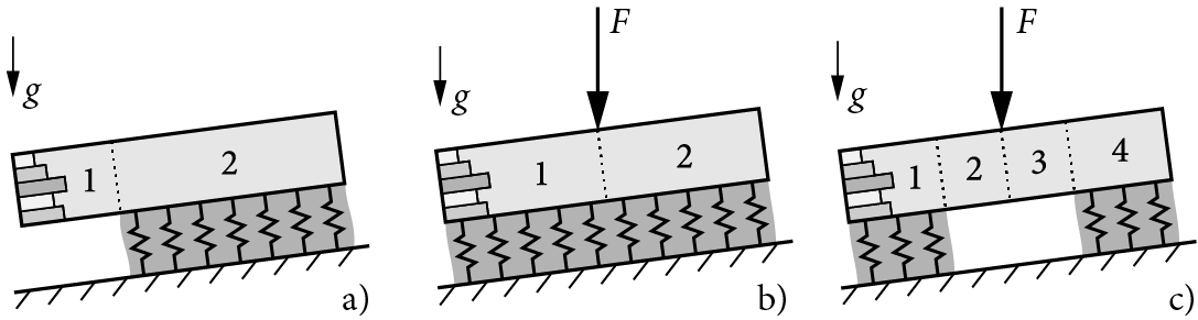
WEAC implements closed-form analytical models for the mechanical analysis of dry-snow slabs on compliant weak layers, the prediction of anticrack onset, and, in particular, allows for the analysis of stratified snow covers. The model covers propagation saw tests (a), and uncracked (b) or cracked (c) skier-loaded buried weak layers.
Cite the repository as:
Rosendahl, P. L., Schneider, J., & Weissgraeber, P. (2022). Weak Layer Anticrack Nucleation Model (WEAC). Zenodo. https://doi.org/10.5281/zenodo.5773113
Read the 📄 white paper for model derivations, illustrations, dimensions, material properties, and kinematics:
- Weißgraeber, P. & Rosendahl, P. L. (2023). A closed-form model for layered snow slabs. The Cryosphere, 17(4), 1475–1496. https://doi.org/10.5194/tc-17-1475-2023
For more background info, please refer to the companion papers:
- Rosendahl, P. L. & Weißgraeber, P. (2020). Modeling snow slab avalanches caused by weak-layer failure – Part 1: Slabs on compliant and collapsible weak layers. The Cryosphere, 14(1), 115–130. https://doi.org/10.5194/tc-14-115-2020
- Rosendahl, P. L. & Weißgraeber, P. (2020). Modeling snow slab avalanches caused by weak-layer failure – Part 2: Coupled mixed-mode criterion for skier-triggered anticracks. The Cryosphere, 14(1), 131–145. https://doi.org/10.5194/tc-14-131-2020
Written in 🐍 Python and built with 💻 Visual Studio Code, 🐙 GitKraken, and 🪐 Jupyter. Note that release v1.0 was written and built in 🌋 MATLAB.
Installation
Install globally using the pip Package Installer for Python
pip install -U weac
or clone the repo
git clone https://github.com/2phi/weac
for local use.
Needs (runtime dependencies are declared in pyproject.toml):
- Python ≥ 3.12
- Numpy ≥ 2.0.1
- Scipy ≥ 1.14.0
- Matplotlib ≥ 3.9.1
- Pydantic ≥ 2.11.7
- Snowpylot ≥ 1.1.5
- snowmicropyn ≥ 1.4.0
Development Setup
This project uses uv for fast Python package management and project handling.
Installing uv
Install uv following the official installation guide:
# On macOS and Linux
curl -LsSf https://astral.sh/uv/install.sh | sh

# Using pip (alternative)
pip install uv
Setting up the development environment
Clone the repository and set up the development environment:
git clone https://github.com/2phi/weac
cd weac

# Install Python 3.12+ if not already available
# uv will automatically use the version specified in .python-version

# For basic setup (if only running the package):
uv sync

# For development (recommended for contributors):
uv sync --extra dev

# Activate the virtual environment
source .venv/bin/activate  # On Windows: .venv\Scripts\activate
Running tests
Run the test suite using uv:
uv run pytest
Code formatting and linting
This project uses ruff for fast Python linting and formatting:
# Format code
uv run ruff format .

# Check for linting issues
uv run ruff check .

# Fix auto-fixable linting issues
uv run ruff check . --fix
Building the package
Build the package for distribution:
# Build wheel and source distribution
uv build

# Install in editable mode for development
uv pip install -e .
Additional uv commands
# Update dependencies
uv sync --upgrade

# Add a new dependency
uv add package-name

# Add a development dependency
uv add --dev package-name

# Show environment info
uv run python --version
uv run pip list
Usage
The following describes the basic usage of WEAC. Please refer to the demo for more examples and read the documentation for details.
Load the module.
import weac
Choose a snow profile from the preconfigured profiles (see dummy_profiles in demo) or create your own using the Layer Pydantic class. One row corresponds to one layer counted from top (below surface) to bottom (above weak layer).
from weac.components import Layer

layers = [
  Layer(rho=170, h=100),  # (1) surface layer
  Layer(rho=190, h=40),   # (2)
  Layer(rho=230, h=130),  #  :
  Layer(rho=250, h=20),
  Layer(rho=210, h=70),
  Layer(rho=380, h=20),   #  :
  Layer(rho=280, h=100)   # (N) last slab layer above weak layer
]
Create a WeakLayer instance that lies underneath the slab.
from weac.components import WeakLayer

weak_layer = WeakLayer(rho=125, h=20)
Create a Scenario that defines the environment and setup that the slab and weak layer will be evaluated in.
from weac.components import ScenarioConfig, Segment

# Example 1: SKIER
skier_config = ScenarioConfig(
    system_type='skier',
    phi=30,
)
skier_segments = [
    Segment(length=5000, has_foundation=True, m=0),
    Segment(length=0, has_foundation=False, m=80),
    Segment(length=0, has_foundation=False, m=0),
    Segment(length=5000, has_foundation=True, m=0),
]  # Scenario is a skier of 80 kg standing on a 10 meter long slab at a 30 degree angle

# Exampel 2: PST
pst_config = ScenarioConfig(
    system_type='pst-',  # Downslope cut
    phi=30,  # (counterclockwise positive)
    cut_length=300,
)
pst_segments = [
    Segment(length=5000, has_foundation=True, m=0),
    Segment(length=300, has_foundation=False, m=0),  # Crack Segment
]  # Scenario is Downslope PST with a 300mm cut
Create a SystemModel instance that combines the inputs and handles system solving and field-quantity extraction.
from weac.components import Config, ModelInput
from weac.core.system_model import SystemModel

# Example: build a model for the skier scenario defined above
model_input = ModelInput(
    weak_layer=weak_layer,
    scenario_config=skier_config,
    layers=custom_layers,
    segments=skier_segments,
)
system_config = Config(
    touchdown=True
)
skier_system = SystemModel(
    model_input=model_input,
    config=system_config,
)
Unknown constants are cached_properties; calling skier_system.unknown_constants solves the system of linear equations and extracts the constants.
C = skier_system.unknown_constants
Analyzer handles rasterization + computation of involved slab and weak-layer properties Sxx, Sxz, etc.
Prepare the output by rasterizing the solution vector at all horizontal positions xsl (slab). The result is returned in the form of the ndarray z. We also get xwl (weak layer) that only contains x-coordinates that are supported by a foundation.
from weac.analysis.analyzer import Analyzer

skier_analyzer = Analyzer(skier_system)
xsl_skier, z_skier, xwl_skier = skier_analyzer.rasterize_solution(mode="cracked")
Gdif, GdifI, GdifII = skier_analyzer.differential_ERR()
Ginc, GincI, GincII = skier_analyzer.incremental_ERR()
# and Sxx, Sxz, Tzz, principal stress, incremental_potential, ...
Visualize the results.
from weac.analysis.plotter import Plotter

plotter = Plotter()
# Visualize slab profile
fig = plotter.plot_slab_profile(
    weak_layers=weak_layer,
    slabs=skier_system.slab,
)

# Visualize deformations as a contour plot
fig = plotter.plot_deformed(
  xsl_skier, xwl_skier, z_skier, skier_analyzer, scale=200, window=200, aspect=2, field="Sxx"
)

# Plot slab displacements (using x-coordinates of all segments, xsl)
plotter.plot_displacements(skier_analyzer, x=xsl_skier, z=z_skier)
# Plot weak-layer stresses (using only x-coordinates of bedded segments, xwl)
plotter.plot_stresses(skier_analyzer, x=xwl_skier, z=z_skier)
Compute output/field quantities for exporting or plotting.
# Compute stresses in kPa in the weaklayer
tau = skier_system.fq.tau(Z=z_skier, unit='kPa')
sig = skier_system.fq.sig(Z=z_skier, unit='kPa')

w = skier_system.fq.w(Z=z_skier, unit='um')
# Example evaluation vertical displacement at top/mid/bottom of the slab
u_top = skier_system.fq.u(Z=z_skier, h0=top, unit='um')
u_mid = skier_system.fq.u(Z=z_skier, h0=mid, unit='um')
u_bot = skier_system.fq.u(Z=z_skier, h0=bot, unit='um')
psi = skier_system.fq.psi(Z=z_skier, unit='deg')
Parsing field profiles into layers
Instead of hand-building Layer lists, WEAC ships parsers in weac.parser that convert common field-profile formats into slope-normal WEAC layers (ordered surface → ground). All parsers expose extract_layers(...) returning (layers, density_methods), so the output plugs directly into ModelInput. See demo/parser_demo.ipynb for side-by-side plots of the three parsers on a co-located Weissfluhjoch pit.
from weac.parser import SMPParser, SnowScopeParser, SnowPilotParser
SnowMicroPen (.PNT) — SMPParser derives density and SSA from the force signal via snowmicropyn's Löwe 2012 shot-noise model plus a parameterization (P2015, CR2020, K2020a, K2020b). Surface and ground are auto-detected at construction. The probe is driven normal to the slope, so recorded depths are already slope-normal and are not scaled by slope angle.
smp = SMPParser("profile.PNT", density_method="CR2020")
# "bin" groups at a fixed thickness; "gradient" cuts on density-gradient jumps
layers, density_methods = smp.extract_layers(method="bin", layer_thickness_mm=20.0)
SnowScope (.csv) — SnowScopeParser reads penetration hardness (kPa) and derives density from a semilog model D = a·ln(F) + b (default HAGENMULLER2018). Layering matches the SMP parser (bin / gradient). SnowScope depths are plumb, so pass slope_angle_deg to scale Layer.h by cos(phi).
scope = SnowScopeParser("profile.csv", density_method="HAGENMULLER2018")
layers, density_methods = scope.extract_layers(method="gradient", gradient_threshold=12.0)

scope_custom = SnowScopeParser(
    "profile.csv",
    semilog_slope=50.0,
    semilog_intercept=100.0,
)
SnowPilot / CAAML (.xml) — SnowPilotParser uses snowpylot to read CAAML snowpits, emitting hand-hardness / density-observation layers. Densities come from measured observations where available, falling back to the Geldsetzer estimate from grain type and hand hardness.
pilot = SnowPilotParser("profile.xml")
# pass a known slope angle to scale plumb depths to slope-normal, e.g.:
# pilot.extract_layers(slope_angle_deg=pilot.pit_slope_angle_deg() or 0.0)
layers, density_methods = pilot.extract_layers()
Roadmap
See the open issues for a list of proposed features and known issues.
v4.0
- Change to scenario & scenario_config: InfEnd/Cut/Segment/Weight
v3.3
- Improved CriteriaEvaluator Optimization (x2 time reduction)
Release history
v3.2.0
- Breaking:
CriteriaEvaluator.evaluate_SteadyStaterewrite uses different inputs and produces different outputs. Two independent configurations are evaluated for tensile failure and energy release rate - Steady-state evaluation uses independent configurations (for tensile and ERR legs)
- Analysis package flatten: Steady State, CoupledCriterion, and Envelopes live in independent files
- Split
LayerandWeakLayerinto separate component models - Jamieson–Johnson slab tensile strength method (
tensile_strength_method="jamieson_johnson") - Weak-layer Young's modulus from Schöttner FC&DH density law (
E_method="schottner_fc_dh") - Lowered weak-layer preset densities to 100/150/200 kg/m³ (within the Schöttner ≤250 kg/m³ range)
v3.1
- Variational model for out-of-plane bending
- Complex terrain through the addition of out-of-plane tilt
- Up, down, and cross-slope cracks
- "generalized" backend with multi-component field support, selectable constitutive models, slab width (b), rotation angle (theta), explicit left/right load vectors, per-segment loading flags, and Mode‑III workflows (GIII).
v3.0
- Refactored the codebase for improved structure and maintainability
- Added property caching for improved efficiency
- Added input validation
- Adopted a new, modular, and object-oriented design
v2.6
- Introduced test suite
- Mitraged from
setup.cfgtopyproject.toml - Added parametrization for collaps heights
v2.5
- Analyze slab touchdown in PST experiments by setting
touchdown=True - Completely redesigned and significantly improved API documentation
v2.4
- Choose between slope-normal (
'-pst','pst-') or vertical ('-vpst','vpst-') PST boundary conditions
v2.3
- Stress plots on deformed contours
- PSTs now account for slab touchdown
v2.2
- Sign of inclination
phiconsistent with the coordinate system (positive counterclockwise) - Dimension arguments to field-quantity methods added
- Improved aspect ratio of profile views and contour plots
- Improved plot labels
- Convenience methods for the export of weak-layer stresses and slab deformations provided
- Wrapper for (re)calculation of the fundamental system added
- Now allows for distributed surface loads
v2.1
- Consistent use of coordinate system with downward pointing z-axis
- Consitent top-to-bottom numbering of slab layers
- Implementation of PSTs cut from either left or right side
v2.0
- Completely rewritten in 🐍 Python
- Coupled bending-extension ODE solver implemented
- Stress analysis of arbitrarily layered snow slabs
- FEM validation of
- displacements
- weak-layer stresses
- energy release rates in weak layers
- Documentation
- Demo and examples
v1.0
- Written in 🌋 MATLAB
- Deformation analysis of homogeneous snow labs
- Weak-layer stress prediction
- Energy release rates of cracks in weak layers
- Finite fracture mechanics implementation
- Prediction of anticrack nucleation
How to contribute
-
Fork the project
-
Initialize submodules
git submodule update --init --recursive
-
Create your feature branch (
git checkout -b feature/amazingfeature) -
Commit your changes (
git commit -m 'Add some amazing feature') -
Push to the branch (
git push origin feature/amazingfeature) -
Open a pull request
Workflows


License
WEAC is licensed under CC BY-NC-SA 4.0


You are free to:
- Share — copy and redistribute the material in any medium or format
- Adapt — remix, transform, and build upon the material for any purpose, even commercially.
Under the following terms:
-
Attribution — You must give appropriate credit, provide a link to the license, and indicate if changes were made. You may do so in any reasonable manner, but not in any way that suggests the licensor endorses you or your use.
-
NonCommercial — You may not use the material for commercial purposes.
-
ShareAlike — If you remix, transform, or build upon the material, you must distribute your contributions under the same license as the original.
Contact
E-mail: mail@2phi.de · Web: https://2phi.de · Project Link: https://github.com/2phi/weac · Project DOI: http://dx.doi.org/10.5281/zenodo.5773113
1 maintainer

Release files for weac 3.3.1
For a detailed explanation of source distributions (sdists) and built distributions (wheels), please see the package formats documentation.
Source distribution (sdist)
| File | Size | Uploaded | |
|---|---|---|---|
| weac-3.3.1.tar.gz | 446.8 kB | Details |
Built distribution (wheel)
| File | Interpreter | ABI | Platform | Reset |
|---|---|---|---|---|
| weac-3.3.1-py3-none-any.whl | Python 3 | none | any | Details |
Total release size: 591.1 kB
Release files / weac-3.3.1.tar.gz
| Download URL | weac-3.3.1.tar.gz |
|---|---|
| Size | 446.8 kB |
| Tags | Source |
|
SHA-256 checksum How to use checksums |
dda3e56bd9798574c49ba9622bfefcdf6d21b978dbcc241f1547d7ca450a12b2
|
|
BLAKE2b-256 checksum How to use checksums |
775f9c5bfe44c9f0f045275b03eb90b3f77405672d0251bed19342890fe17954
|
| Upload date | |
|
Uploaded using Trusted Publishing? What is trusted publishing? |
No |
| Uploaded via |
twine/6.2.0 CPython/3.12.10
|
Release files / weac-3.3.1-py3-none-any.whl
| Download URL | weac-3.3.1-py3-none-any.whl |
|---|---|
| Size | 144.2 kB |
| Tags | Python 3 |
|
SHA-256 checksum How to use checksums |
07e4163b349ce1ca5b79f58266f9d02cea6f22db1dd2b3908dc9481ca475587d
|
|
BLAKE2b-256 checksum How to use checksums |
dda6fea3c525c7d66284bebf53fcaeac5c29adf8240f16a9b494507fd0777a98
|
| Upload date | |
|
Uploaded using Trusted Publishing? What is trusted publishing? |
No |
| Uploaded via |
twine/6.2.0 CPython/3.12.10
|














