Hurst exponent estimation using Whittle's method

Project description


Overview
This module implements Whittle's likelihood estimation method for determining the Hurst exponent of a time series. The method fits the theoretical spectral density to the periodogram computed from the time series realization. This implementation includes spectral density approximations for fractional Gaussian noise (increments of fractional Brownian motion) and ARFIMA processes.
The Hurst exponent ($H$) controls the roughness, self-similarity, and long-range dependence of fBm paths:
- $H\in(0,0.5):~$ anti-persistent (mean-reverting) behavior.
- $H=0.5:~ \mathrm{fBm}(H)$ is the Brownian motion.
- $H\in(0.5,1):~$ persistent behavior.
Features
- Spectral density options:
fGn(This is the current default option, corresponding to fGn_Paxson, with K=10)arfimafGn_PaxsonfGn_HurwitzfGn_truncationfGn_Taylor
- A flexible interface that supports custom spectral density callback functions.
- Good performance both in terms of speed and accuracy.
- Included generators for fBm and ARFIMA.
Installation
pip install whittlehurst
Usage
Whittle for fBm and fGn
import numpy as np
from whittlehurst import whittle, fbm

# Original Hurst value to test with
H=0.42

# Generate an fBm realization
fBm_seq = fbm(H=H, n=10000)

# Calculate the increments (the estimator works with the fGn spectrum)
fGn_seq = np.diff(fBm_seq)

# Estimate the Hurst exponent
H_est = whittle(fGn_seq)

print(f"Original H: {H:0.04f}, estimated H: {H_est:0.04f}")
TDML for fGn
The Time-Domain Maximum Likelihood (TDML) method estimates $H$ from fGn observations by fitting the likelihood function directly in the time domain. TDML performs a similar root finding as Whittle's method, but Whittle operates in the frequency domain. Despite significant optimizations TDML remains much slower than Whittle. TDML offers marginally improved accuracy, especially at the edges of the Hurst parameter range.
Usage:
import numpy as np
from whittlehurst import tdml, fbm

# Original Hurst value to test with
H=0.42

# Generate an fBm realization
fBm_seq = fbm(H=H, n=10000)

# Calculate the increments
fGn_seq = np.diff(fBm_seq)

# Estimate the Hurst exponent
H_est = tdml(fGn_seq)

print(f"Original H: {H:0.04f}, estimated H: {H_est:0.04f}")
ARFIMA
import numpy as np
from whittlehurst import whittle, arfima

# Original Hurst value to test with
H=0.42

# Generate a realization of an ARFIMA(0, H - 0.5, 0) process.
arfima_seq = arfima(H=H, n=10000)

# No need to take the increments here
# Estimate the "Hurst exponent" using the ARFIMA spectrum
H_est = whittle(arfima_seq, spectrum="arfima")

print(f"Original H: {H:0.04f}, estimated H: {H_est:0.04f}")
Performance
Compared to other methods
Our Whittle-based estimator offers a compelling alternative to traditional approaches for estimating the Hurst exponent. In particular, we compare it with:
-
R/S Method: Implemented in the hurst package, this method has been widely used for estimating $H$.
-
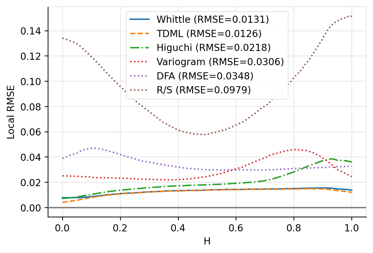
Higuchi's Method: Available through the antropy package, it performs quite well especially for smaller $H$ values, but its performance drops when $H\rightarrow 1$.
-
DFA: Detrended Fluctuation Analysis is a popular Hurst estimator robust for non-stationary processes (this robustness is not required in the below tests). Available through the nolds package.
-
Variogram: Our variogram implementation of order $p = 1$ (madogram) accessible as
from whittlehurst import variogram. -
TDML: Our TDML implementation.
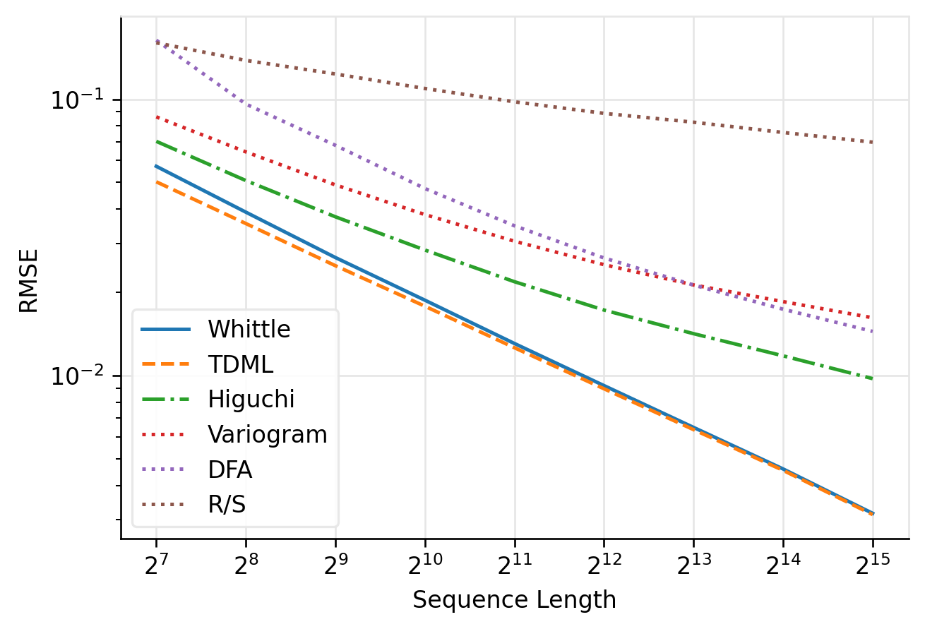
Inference times represent the computation time per input sequence, and were calculated as: $t = w\cdot T/k$, where $k=100000$ is the number of sequences, $w=32$ is the number of workers (processing threads), and $T$ is the total elapsed time. Single-thread performance is likely superior, the results are mainly comparative.
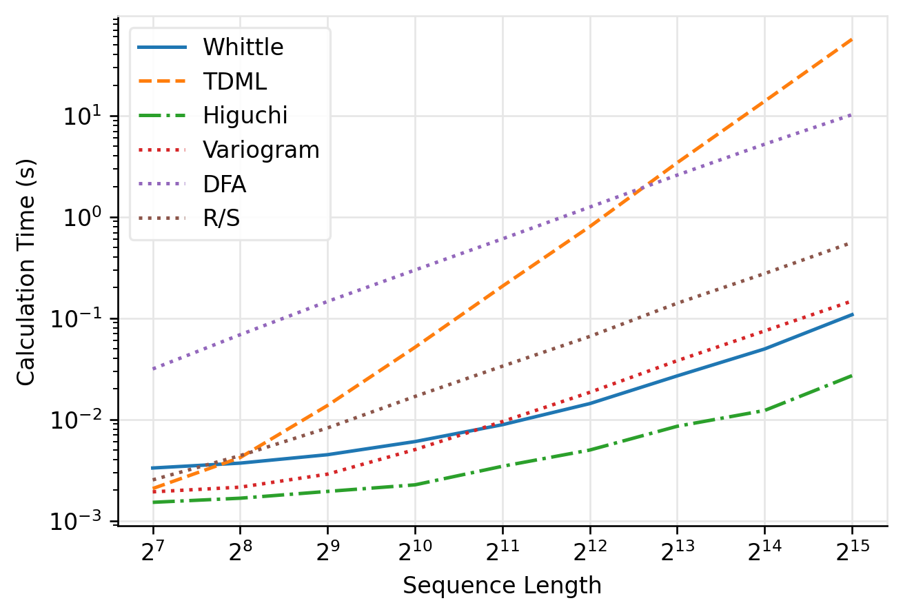
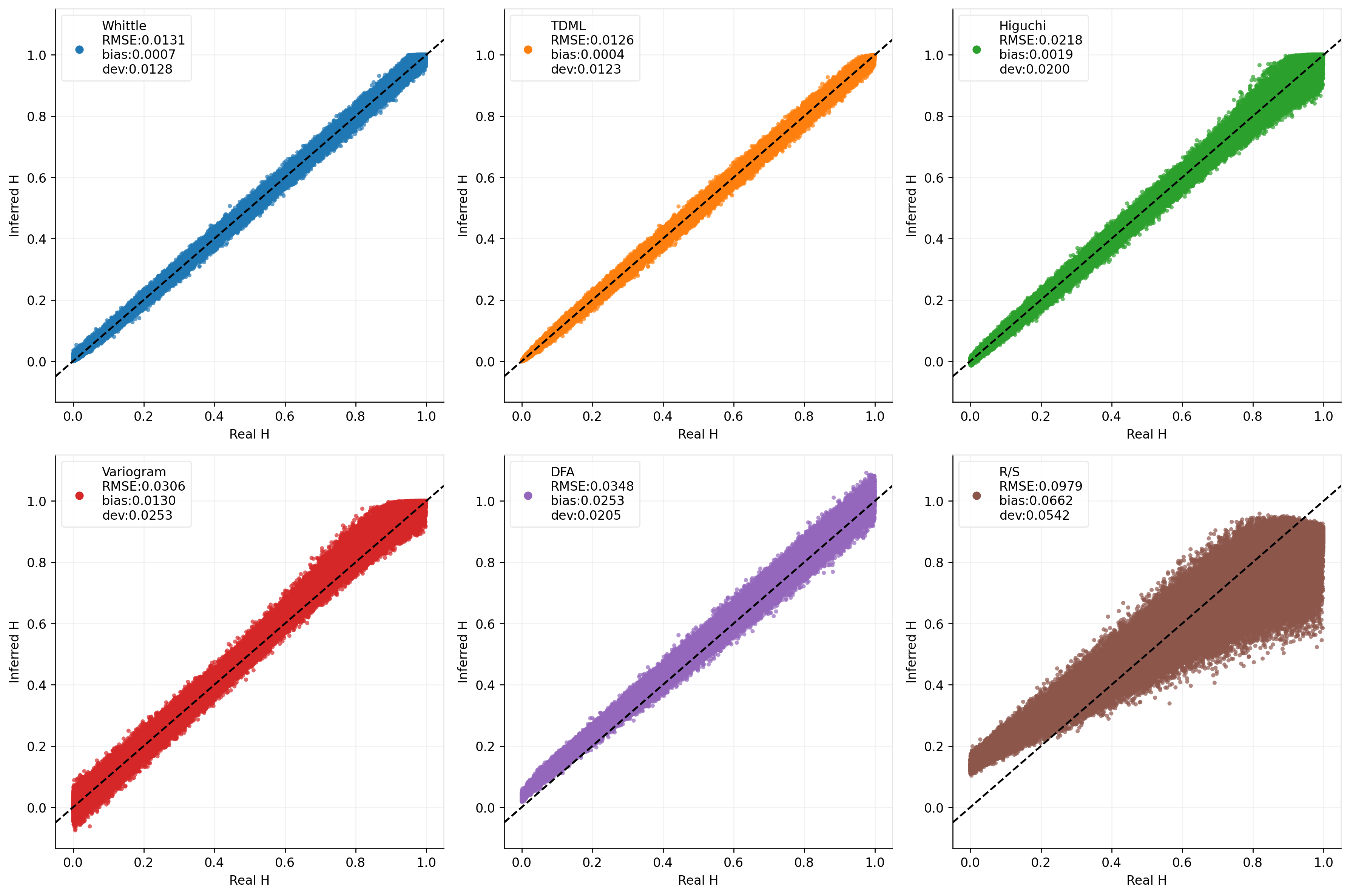
The following results were calculated on $100000$ fBm realizations of length $n=2048$.
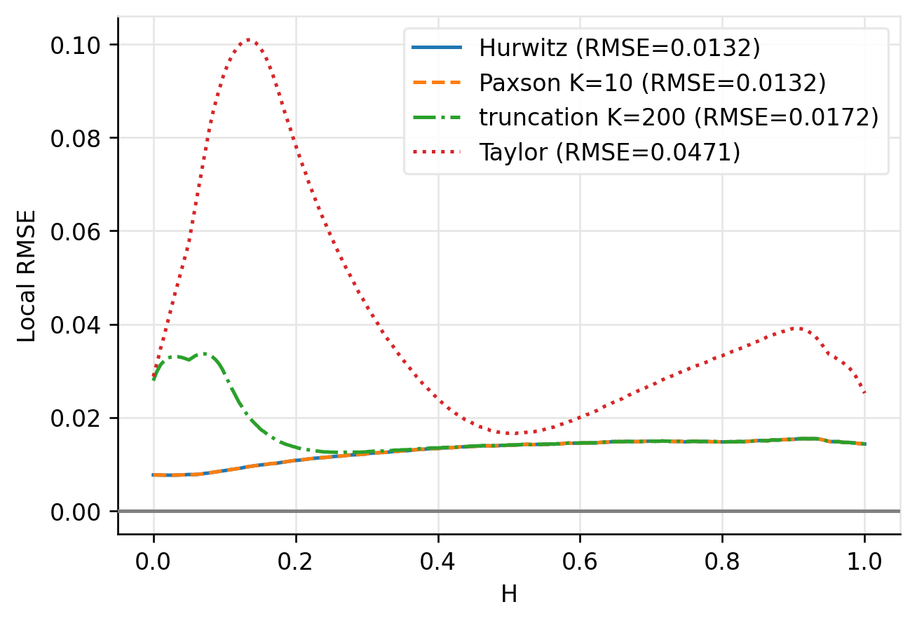
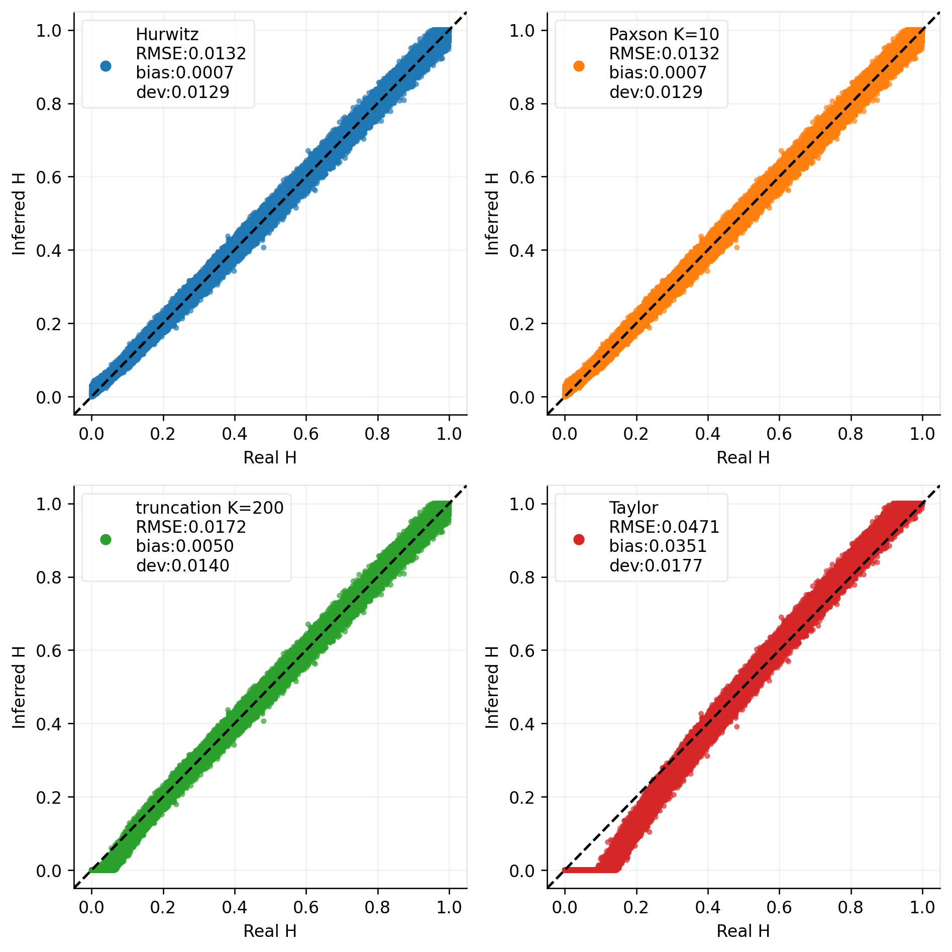
fGn spectral density approximations
The fGn spectral density calculations recommended by Shi et al. are accessible within our package:
fGnorfGn_Paxson: The default recommended spectral model. Uses Paxson's approximation with a configurable parameterK=10.fGn_Hurwitz: Relies on the gamma function and the Hurwitz zeta function $\zeta(s,q)=\sum_{j=0}^{\infty}(j+q)^{-s}$ from scipy.fGn_truncation: Approximates the infinite series by a configurable truncationK=200.fGn_Taylor: Uses a Taylor series expansion to approximate the spectral density at near-zero frequency.
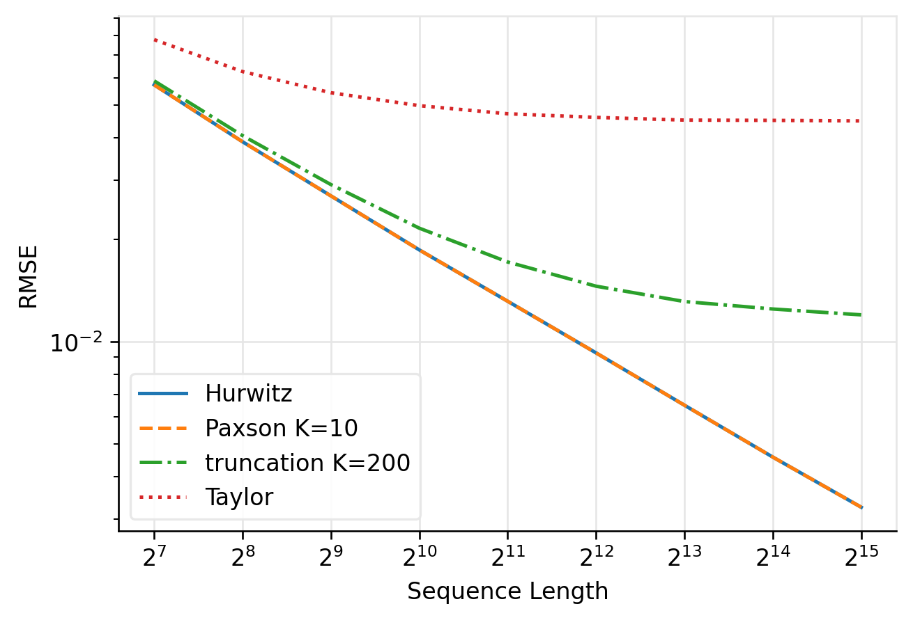
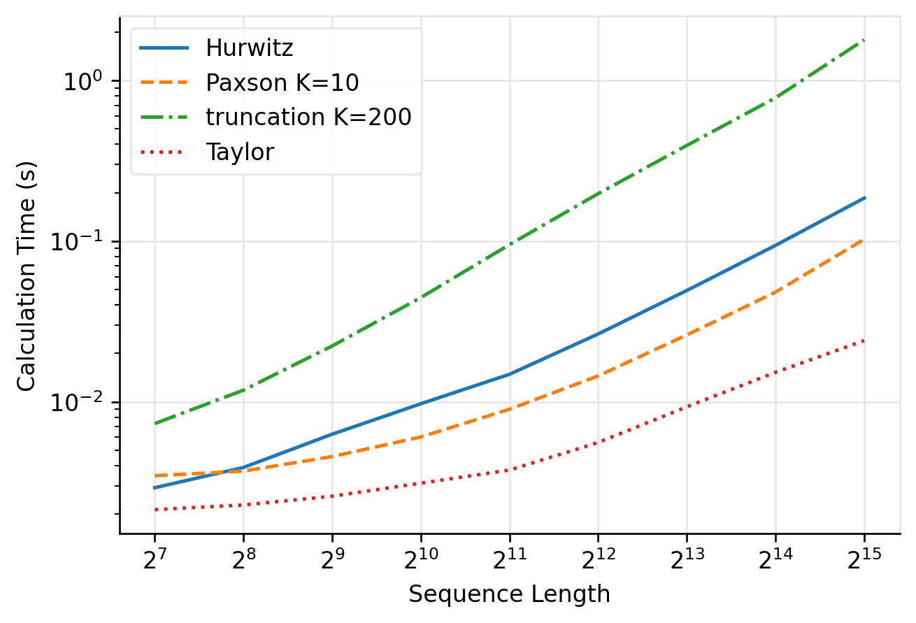
The following results were calculated on $100000$ fBm realizations of length $n=2048$.
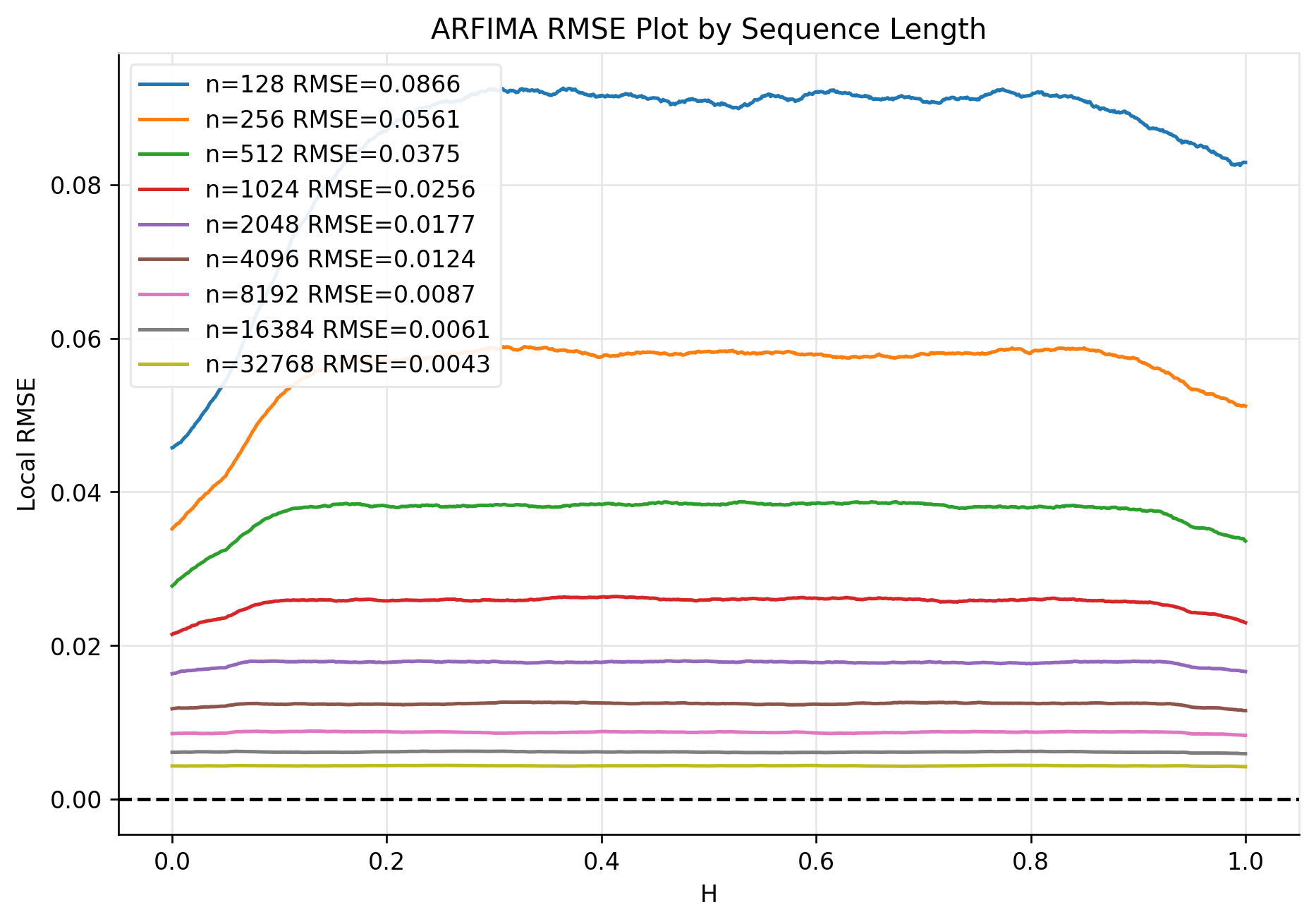
ARFIMA
For the $\text{ARFIMA}(0, H - 0.5, 0)$ process, the spectral density calculation is simpler. With terms independent from $H$ or $\lambda$ omitted, we use:
$g(\lambda,H) = (2\cdot\sin(\lambda/2))^{1 - 2H}$
How to Cite
@misc{csanády2025whittlehurstpythonpackageimplementing,
      title={$whittlehurst$: A Python package implementing Whittle's likelihood estimation of the Hurst exponent},
      author={Bálint Csanády and Lóránt Nagy and András Lukács},
      year={2025},
      eprint={2506.01985},
      archivePrefix={arXiv},
      primaryClass={stat.CO},
      url={https://arxiv.org/abs/2506.01985},
}
References
-
The initial implementation of Whittle's method was adapted from:
https://github.com/JFBazille/ICode/blob/master/ICode/estimators/whittle.py
-
For further details on spectral density models for fractional Gaussian noise, refer to:
Shuping Shi, Jun Yu, and Chen Zhang. Fractional gaussian noise: Spectral density and estimation methods. Journal of Time Series Analysis, 2024. https://onlinelibrary.wiley.com/doi/full/10.1111/jtsa.12750
License
This project is licensed under the MIT License (c) 2025 Bálint Csanády, aielte-research. See the LICENSE file for details.


Download files
Download the file for your platform. If you're not sure which to choose, learn more about installing packages.
Source Distribution
Built Distribution
Filter files by name, interpreter, ABI, and platform.
If you're not sure about the file name format, learn more about wheel file names.
Copy a direct link to the current filters
File details
Details for the file whittlehurst-1.4.tar.gz.
File metadata
- Download URL: whittlehurst-1.4.tar.gz
- Upload date:
- Size: 14.9 kB
- Tags: Source
- Uploaded using Trusted Publishing? No
- Uploaded via: twine/6.2.0 CPython/3.12.12
File hashes
| Algorithm | Hash digest | |
|---|---|---|
| SHA256 |
3d0fd1f9659c75b130c433eb8877599bde3225561b7dd3d1e2eaded86fcf8fd5
|
|
| MD5 |
35901af3e800e48ef351b82c43d622c6
|
|
| BLAKE2b-256 |
40ffdb9385b60ddb44227b4373a4b43159c1d0583e51378bfe657a5d6b3e8c90
|
File details
Details for the file whittlehurst-1.4-py3-none-any.whl.
File metadata
- Download URL: whittlehurst-1.4-py3-none-any.whl
- Upload date:
- Size: 13.2 kB
- Tags: Python 3
- Uploaded using Trusted Publishing? No
- Uploaded via: twine/6.2.0 CPython/3.12.12
File hashes
| Algorithm | Hash digest | |
|---|---|---|
| SHA256 |
cba916d20642ba8f96c80daa3fecd7d67bdae6b9e0424b90dcbbda7ac8ffbcec
|
|
| MD5 |
bd2ece8884f310e08d11064d0f5cbe5f
|
|
| BLAKE2b-256 |
eebbe3d002d419c353b37a9b3a7a5dfa61d7c7290bcc51e3b6774b698adb1e37
|


