
Whole History Rating (WHR) Python Implementation
This Python library is a conversion from the original Ruby implementation of Rémi Coulom's Whole-History Rating (WHR) algorithm, designed to provide a dynamic rating system for games or matches where players' skills are continuously estimated over time.
The original Ruby code is available here at goshrine.
Installation
To install the library, use the following command:
pip install whole-history-rating
How well does it actually work?
WHR is benchmarked against the two reference implementations it is usually
compared to — KickScore and
TrueSkill Through Time —
by actually running them, on the same data, under the same protocol, scored
with the same metric. Everything below is reproducible from
benchmarks/; the full write-up, method and caveats are in
benchmarks/REPORT.md.
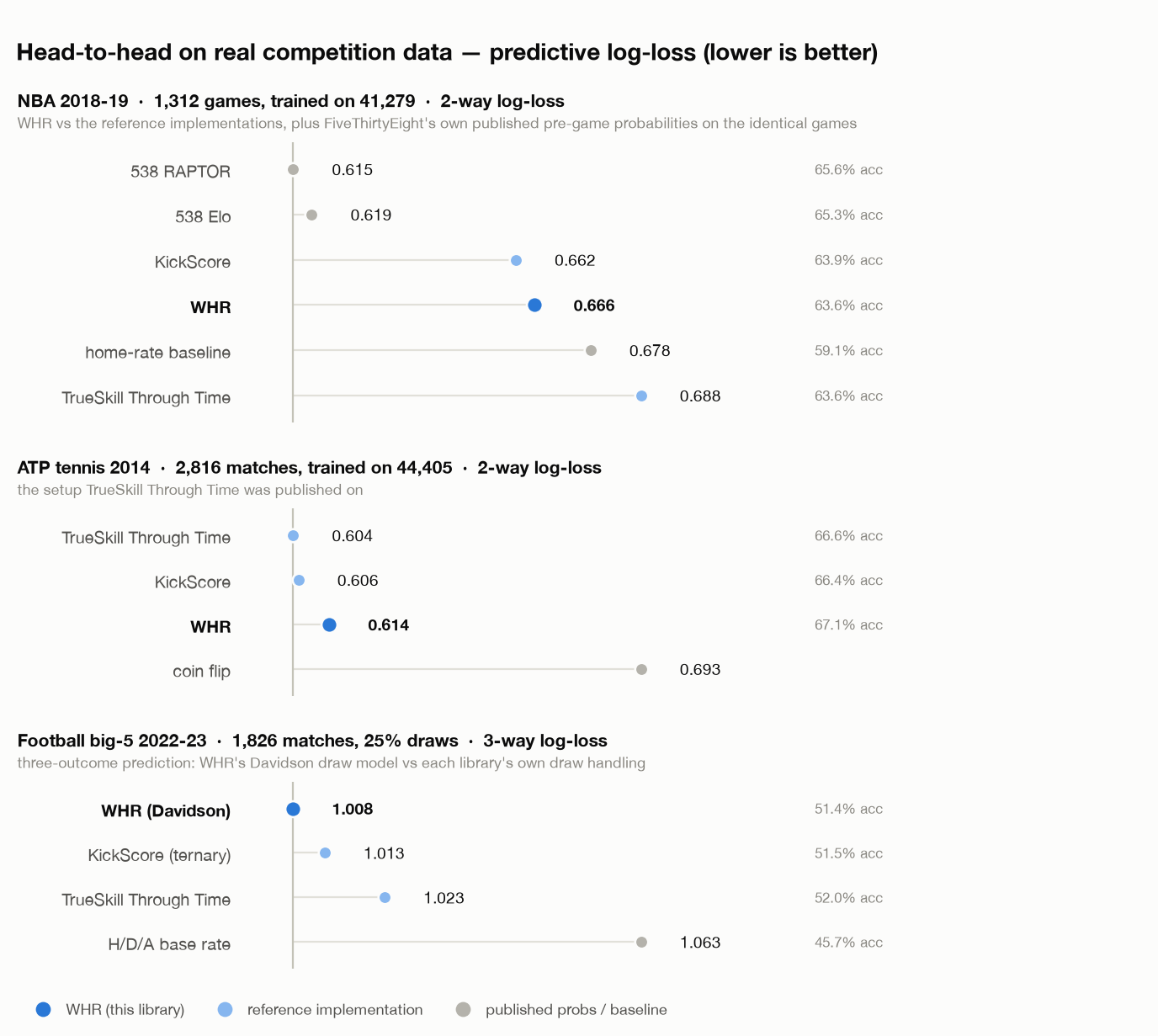
Each system is fitted only on matches played before the test season, and every one of its hyper-parameters — including the competitors' probability-scale knobs, not just their dynamics knobs — is tuned on a separate validation season. Grids were widened until no optimum sat on a grid edge, so no system is reported at a value the grid merely failed to reach.
| Benchmark | Test set | WHR | KickScore | TrueSkill Through Time |
|---|---|---|---|---|
| NBA (FiveThirtyEight) | 2018-19, n=1312 | 0.666 · 63.6% | 0.662 · 63.9% | 0.688 · 63.6% |
| ATP tennis (Sackmann) | 2014, n=2816 | 0.614 · 67.1% | 0.606 · 66.4% | 0.604 · 66.6% |
| Football big-5, 3-way | 2022-23, n=1826 | 1.008 · 51.4% | 1.013 · 51.5% | 1.023 · 52.0% |
Log-loss in nats, lower is better; accuracy after it. Four things worth pulling out, including the ones that do not flatter this library:
- No system wins outright, and the spread is small. WHR takes the football benchmark, KickScore the NBA, TTT the tennis. WHR is never more than 1.5% behind whichever system leads (0.6% on the NBA, 1.5% on tennis), and the full best-to-worst spread stays under 4% on every sport. If you are choosing a library, this benchmark is not the reason to pick one: API, dependencies and speed will matter more than a hundredth of a nat.
- WHR is the strongest of the three at three-outcome prediction. Its
Davidson draw model is fitted from the data (here ν≈0.79) rather
than approximated, and it beats KickScore's ternary
marginand TTT'sp_drawon exactly the same matches. This is the one benchmark where the modelling choice, not the tuning, decides the result. - WHR trades calibration for ranking on two-outcome sports. On tennis it has
the best accuracy of the three (67.1%) and the worst log-loss: it ranks
players at least as well but is overconfident about it. Passing
account_for_uncertainty=Truetoprobability_future_matchrecovers a real part of that gap — on the validation season the sweep selects on, 0.6119 → 0.6094 for tennis and 0.6577 → 0.6549 for the NBA — and is recommended whenever you consume the probabilities rather than the ordering.win_draw_loss_probabilitiestakes the same option; every number in the table above is scored with whichever setting its validation season chose, which wasTrueon all three sports. It buys much less on three outcomes (1.0085 → 1.0083 on football's validation season) because that hedge compresses the win/loss odds rather than moving mass toward the draw. - A domain-specific model still beats all three. FiveThirtyEight's published pre-game probabilities score 0.615 (RAPTOR) and 0.619 (Elo) on the identical 1,312 games, against 0.662–0.688 for the general-purpose systems. RAPTOR sees rosters, injuries and travel; WHR, KickScore and TTT see only who beat whom, and when. That gap is the value of domain features, not a defect of the algorithms — but it is worth knowing before deploying any of them as a forecaster.
The advantages WHR reports are learned, not assumed: given only wins and losses it put the NBA home-court edge at +98 elo (the accepted value is ≈+100) and the football home edge at +79 elo, alongside a draw tendency ν≈0.79.
The ratings are historically recognisable
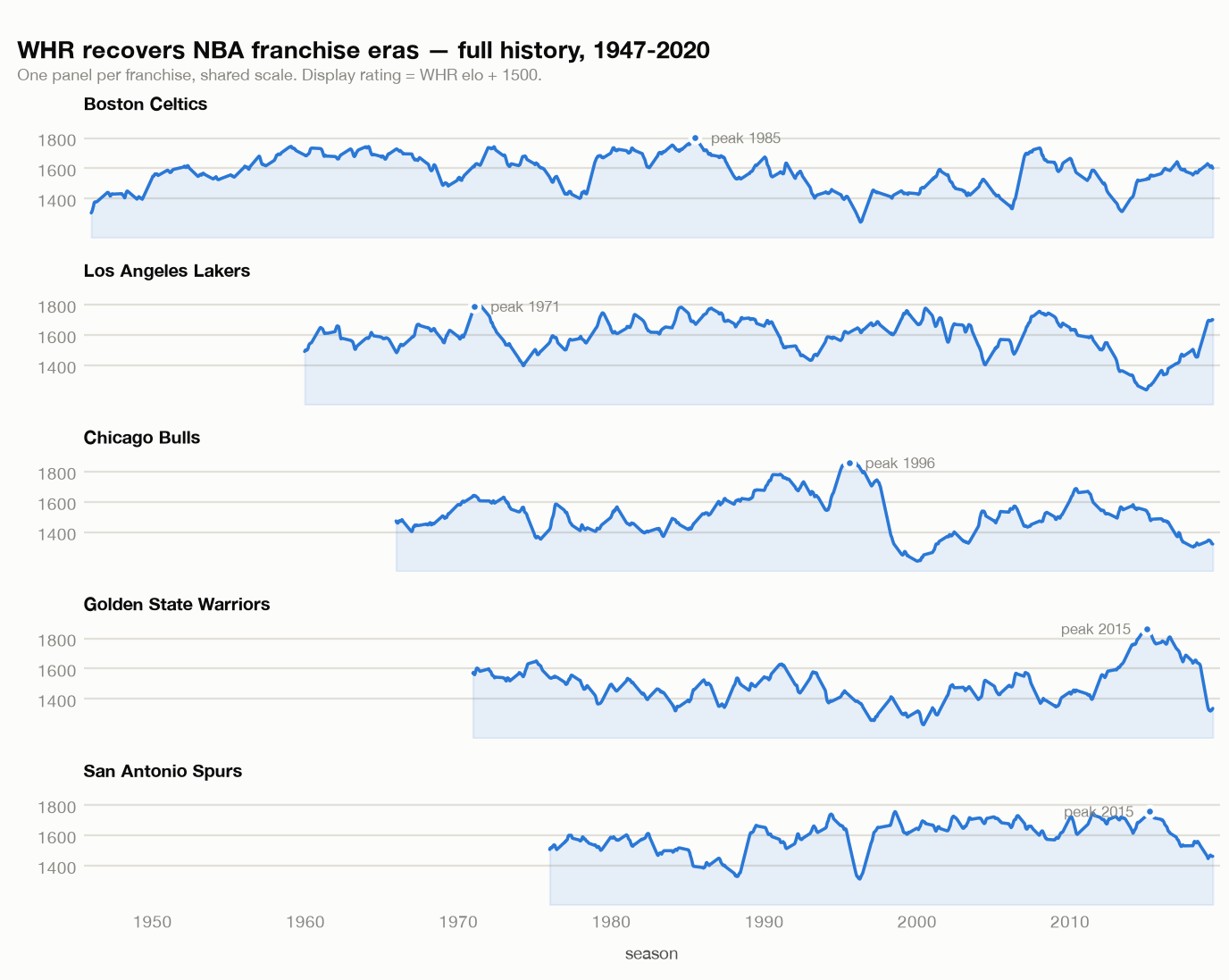
Fitted on the full 1947-2020 NBA history, WHR reproduces the eras a basketball fan would name: the Celtics' long dominance, the Bulls peaking in 1996, the Warriors' spike in 2015, the Spurs' Duncan-era plateau.
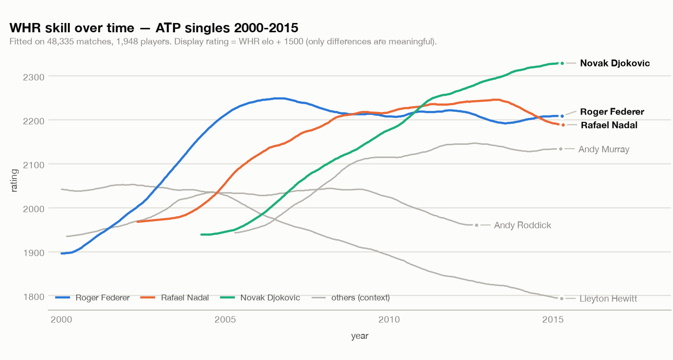
And on ATP tennis, the Federer → Nadal → Djokovic succession falls out of the match results alone:
What this is and is not. KickScore and TrueSkill Through Time are run locally from their own packages, so the three systems share a training prefix, a validation season, a test season, a time unit and a metric — differences in data vintage or train/test split cannot explain the gaps. What it is not is a reproduction of the reference papers' own published numbers, which use different splits and preprocessing. Three protocol decisions are judgement calls worth reading before quoting these figures: cold-start players are answered from each library's own prior, home advantage is expressed in each library's own idiom, and each system gets a fixed convergence budget rather than a matched wall-clock. All three, plus every hyper-parameter grid, are documented in
benchmarks/REPORT.md.
Usage
Basic Setup
Start by importing the library and initializing the WHR object:
from whr import WHR

whr = WHR()
The class used to be called
Base. That name still works as a deprecated alias (it emits aDeprecationWarning); preferWHRin new code.
Creating Games
Add games to the system using create_game() method. It takes the names of the black and white players, the winner ("B" black, "W" white, or "D" draw), the day number, a handicap key, and an optional komi key.
whr.create_game("shusaku", "shusai", "B", 1, 0)
whr.create_game("shusaku", "shusai", "W", 2, 0)
whr.create_game("shusaku", "shusai", "W", 3, 0)
handicapis a category key, not a fixed elo bonus — its advantage is learned from the data (or pinned). See "Handicap and komi" below; use0for an even game. (This changed in 3.0.0 — in 2.x it was a raw elo constant.)- The day is a day index counted from an origin you choose, and it defines a player's playing days: two games with the same value share one rated day. Fractional values are allowed (the time prior uses
|Δdays| · w2), and an integral float is narrowed toint, so1.0and1are the same day rather than two. Non-numbers, booleans and NaN/infinity are rejected at this call. Keep the span compact — see the note under "Removing Rating Drift" about epoch timestamps. "D"records a draw — see "Draws".komiis opt-in (as of 3.1.0): the defaultNonemodels no komi at all. Pass a value to model a white-side (komi) advantage for that game, whose category is learned like the handicap:
# Standalone illustration — NOT part of the three-game example above.
other = WHR()
other.create_game("alice", "bob", "B", 1, 0, komi=7.5)
(An extras={"komi": …} dict is still accepted for backward compatibility. Before 3.1.0 a komi of 6.5 was assumed for every game and estimated; pass komi=6.5 to reproduce that.)
About the numbers in this README. Every output shown below is the real, current output of the snippet above it. The
shusaku/shusaifigures all come from exactly the three games just created, followed bywhr.iterate(50)— so you can paste those four lines and reproduce them. Ratings changed in 3.0.0 and again in 3.1.0, so numbers copied from older docs will not match.
Refining Ratings Towards Stability
To achieve accurate and stable ratings, the WHR algorithm allows for iterative refinement. This process can be controlled manually or handled automatically to adjust player ratings until they reach a stable state.
Manual Iteration
For manual control over the iteration process, specify the number of iterations you wish to perform. This approach gives you direct oversight over the refinement steps.
whr.iterate(50)
This command will perform 50 iterations, incrementally adjusting player ratings towards stability with each step.
Automatic Iteration
For a more hands-off approach, the algorithm can automatically iterate until the Elo ratings stabilize within a specified precision. Automatic iteration is particularly useful when dealing with large datasets or when seeking to automate the rating process.
whr.auto_iterate(time_limit=10, precision=1e-3, batch_size=50)
time_limit(optional): Sets a maximum duration (in seconds) for the iteration process. IfNone(the default), the algorithm will run indefinitely until the specified precision is achieved.precision(optional): Defines the desired level of accuracy for the ratings' stability. The default value is0.001. Convergence is measured on the gradient infinity-norm (the largest absolute gradient component across all player-days, in natural-rating units); iteration stops once that value drops below this threshold.batch_size(optional): Determines the number of iterations to perform before checking for convergence and, if atime_limitis set, before evaluating whether the time limit has been reached. The default is50(raised from10in 3.5.0). Checking is not free:max_gradient_norm()costs about 0.44 of an iteration and, more importantly, clears every game-term cache, so the first iteration after each check has to repopulate it. Reaching a1e-4target on ATP 2000–2006 took 165 s at5, 132 s at10, 115 s at25, 109 s at50, then 130 s at100— where overshooting the target by up tobatch_size - 1wasted iterations starts to dominate. Lower it if you need atime_limithonoured promptly.
This automated process allows the algorithm to efficiently converge to stable ratings, adjusting the number of iterations dynamically based on the complexity of the data and the specified precision and time constraints.
precisionis a gradient threshold, not an elo tolerance — and the default is a good place to stop. Measured on ATP 2000–2013 (44,405 games, 1,842 players) fitted to each target in turn, scoring the held-out 2014 season, and repeated with the games inserted in a shuffled order:
precisioniterations held-out log-loss elo spread across insertion orders 1e-2160 0.616521 5.86 5e-3320 0.614102 2.97 1e-3(default)720 0.613530 0.25 1e-41330 0.613592 0.06 1e-51940 0.613602 0.006 1e-62550 0.613603 0.0006 Predictive quality bottoms out at the default: past
1e-3the loss moves by under1e-4, which is noise on a 2,816-match test set, while the cost rises 1.9× to 3.5×. Looser is measurably worse —1e-2costs 0.003 nats.Tightening buys stability of the rating values, not accuracy: ratings shift by tens of elo between
1e-3and1e-4and settle to hundredths by1e-5. Ask for1e-5if you publish rating numbers and need them stable run to run; stay at the default if you consume predictions.Convergence speed is dataset-shaped, not just size-shaped. The NBA base (41,279 games, 37 teams, 14-day bins) reaches
1e-3in 230 iterations but needs 5,430 for1e-4and cannot reach1e-5inside 900 s — while its held-out loss is flat to five decimals across the whole range. Raiseprecision, or acceptstable=False, rather than assuming a tighter target is always reachable.
Performance. Cost scales with the number of (player, distinct day) pairs rather than with the number of games: each player solves its own tridiagonal system over its own rated days. Two datasets of the same size can therefore differ by an order of magnitude — 41k NBA games over 37 teams in 14-day bins fits in ~4 s, while 44k ATP matches over 1,842 players at day granularity takes ~51 s. If a fit is slower than you expect, coarsen the time unit (bin days into weeks or fortnights) and retune w2 to match: that is the single biggest lever.
The per-game hot paths are batched where batching pays and left in plain Python where it does not — a numpy call costs ~2.5 µs regardless of size, so on the one-to-three games a typical player-day carries, a loop is 10–16× faster. The threshold is internal and a test requires both paths to agree, so it cannot change a result.
Viewing Ratings
Retrieve and view player ratings, which include the day number, elo rating, and uncertainty:
# Continuing the three-game example (B, W, W) after whr.iterate(50):
print(whr.ratings_for_player("shusaku"))
# Output (one (day, elo, uncertainty) tuple per playing day):
#   [(1, -50, 0.26),
#    (2, -51, 0.26),
#    (3, -52, 0.26)]

print(whr.ratings_for_player("shusai"))
# Output:
#   [(1, 50, 0.26),
#    (2, 51, 0.26),
#    (3, 52, 0.26)]
Shusaku lost two of the three games, so he settles ~100 elo below Shusai. The elo values are rounded to integers and the uncertainty to two decimals.
Why are the ratings centred on 0, and can I make them look like "real" elo? WHR estimates relative strength: every player's first day is softly anchored toward 0 elo, so an average player sits near 0 and weaker ones go negative. Only rating differences are meaningful — they are the only thing the win probability uses. Adding a constant to every rating therefore changes no prediction at all, which is exactly how goratings-style scales are produced:
OFFSET = 1500
shifted = [(day, elo + OFFSET, unc) for day, elo, unc in whr.ratings_for_player("shusaku")]
Better, since 3.5.0, let the library hold the scale: set
display_offsetand every display surface applies it, while nothing is written back into the model.whr.config["display_offset"] = 1500 whr.ratings_for_player("shusaku") # elo shifted whr.probability_future_match("shusaku", "shusai", 0) # unchanged — differences onlyA fixed
+1500is arbitrary, though: ratings drift across eras, so the same constant means different things in 1950 and 2020.display_offset_for()derives one from an anchoring rule instead — it returns the value without applying it, so you can inspect it first:whr.config["display_offset"] = whr.display_offset_for(target=1500) # field mean whr.config["display_offset"] = whr.display_offset_for(target=2000, player="shusai") # one playerDo not write the offset into the model by hand. Assigning
day.elo += OFFSETalso leaves predictions unchanged, but the offset is not a fixed point of the fit: the first-day anchor pulls ratings back toward 0, so a lateriterate()erodes it silently — an added 1500 decays to roughly 100 over 500 further iterations.If the spread itself is too narrow, lower
initial_prior_wins(see "Optional Configuration") so weakly-connected players are pulled less toward the centre.
Querying an unknown player raises a ValueError. Before iterate() has run,
uncertainties are the sentinel -1 — not a standard deviation, but "not
computed yet"; reading them emits an UncomputedUncertaintyWarning once per
instance. (rating_difference, rating_covariance and rating_change raise a
ValueError in that same state rather than returning a sentinel.)
The uncertainty is a variance in natural log units, not elo. The
0.26above is not "±0.26 elo": its elo standard error issqrt(0.26) × 400/ln(10)= 88.6 elo, a factor of ~340 apart — which is a real trap in a column of elo values. Setconfig["display_uncertainty"] = "elo"to have this column reported as an elo standard error instead (the default stays"variance"for backward compatibility).rating_differencehas always reported elo.
Ratings read after adding games are out of date.
create_gameandload_gamesonly record; nothing is re-estimated untiliterate()orauto_iterate()runs. Reading in between returns the previous fit, and the error is not small — adding results to a day a player already had moved one rating by 464 elo once re-fitted, while the stale value and its uncertainty looked entirely plausible.max_gradient_norm()is not a reliable check either: it can sit at2e-3throughout. Since 3.5.0 such a read emits aStaleFitWarning, andgames_since_last_fitreports the count.
To get the underlying Player object itself (for direct access to its days,
each day's elo / gamma(), etc.), use player_by_name(). Note it creates
the player if the name is unknown (unlike ratings_for_player, which raises):
player = whr.player_by_name("shusaku")
[(d.day, round(d.elo, 1)) for d in player.days]
# d.elo is a property holding the unrounded value:
#   [(1, -49.8), (2, -51.1), (3, -51.7)]
You can also view or retrieve all ratings in order:
whr.print_ordered_ratings(current=False)  # Set `current=True` for the latest rankings only.
ratings = whr.get_ordered_ratings(current=False, compact=False)  # Set `compact=True` for a condensed list.
Inspecting the Fit
log_likelihood() returns the model's total log-posterior (game likelihood + the first-day prior + the Gaussian Wiener prior over time, and the Davidson draw term when draws are present). It increases as iterate() converges, so it is a handy convergence/diagnostic signal:
whr.log_likelihood() # -> 0.33010610615918456 (three-game example, after iterate(50))
Only the direction is meaningful: higher is a better fit. Note the value is a log density, not a log probability, so it is not bounded above by 0 and can legitimately be positive (as here) — compare it across iterations of the same base, never across different bases.
max_gradient_norm() returns the largest gradient infinity-norm across all player-days (plus the estimated handicap/komi and draw-tendency parameters) — the exact quantity auto_iterate(precision=...) tests. It is the most direct convergence gauge; near 0 means converged:
whr.max_gradient_norm() # -> 9.54e-05 (well under the default 1e-3 precision)
For the win probability of a specific recorded game (rather than a hypothetical match-up), use the Game object returned by create_game:
game = whr.create_game("shusaku", "shusai", "B", 1, 0)
whr.iterate(50)
game.white_win_probability()  # and game.black_win_probability()
game.prediction_score()       # 1.0 if the model's favourite actually won, 0.0 if not, 0.5 on a coin-flip
In normal use ratings always converge to finite values. Only a genuinely non-finite result (e.g. a pathological input) raises whr.utils.UnstableRatingException; it is exported for except handling but should not occur in practice.
Predicting Match Outcomes
Only players linked by a chain of games are comparable. WHR estimates relative strength, so two groups that never meet — separate leagues, disjoint eras, a multi-federation pool — are each anchored toward 0 elo independently, and their numbers look comparable while sitting on different scales. A cross-group prediction is not merely uncertain, it is unfounded: in a base where an undefeated player in one pool faced an evenly-matched player from another, the library answered 0.99 on no shared game whatsoever. Since 3.5.0 such a call emits a
DisconnectedPlayersWarning, andconnected_components()lists the groups (largest first) so you can check:groups = whr.connected_components() # [frozenset({...}), frozenset({...})]Either rate each pool separately, or add the fixtures that actually link them.
Predict the outcome of future matches, including between non-existent players:
# Example of predicting a future match outcome. It is a pure query: it does
# not print anything, and unknown players are treated as an even (gamma = 1)
# reference without being added to the base.
probability = whr.probability_future_match("shusaku", "shusai", 0)
print(f"Win probability: shusaku: {probability[0]*100:.2f}%; shusai: {probability[1]*100:.2f}%")
# Output (three-game example, after iterate(50)):
#   Win probability: shusaku: 35.50%; shusai: 64.50%
That 35.50% is exactly the Bradley-Terry probability implied by the 103.74 elo
gap between the two players' latest ratings (-51.69 and +52.05):
1 / (1 + 10**(103.74/400)).
Uncertainty
Beyond the per-day uncertainty from ratings_for_player, three methods turn
that raw variance into comparisons and predictions. All of them report elo
and require iterate()/auto_iterate() to have run first (an unrated player
raises ValueError).
Comparing two players. A player's own elo doesn't by itself say how
confidently they're ahead of a rival — the difference between the two is
the comparable quantity, given by rating_difference():
whr = WHR()
for day in range(1, 11):
    whr.create_game("north", "referee", "B", day, 0)  # north usually wins
for day in range(1, 11):
    whr.create_game("south", "referee", "W", day, 0)  # south usually loses
whr.auto_iterate()

whr.rating_difference("north", "south")
# {'difference': 1056.95, 'std_error': 85.74,
#  'confidence_interval_95': (888.9, 1224.99)}
This is an approximation: WHR never computes cross-player covariance, so
the difference's variance is Var(a) + Var(b) (an independence assumption).
Two players who have played each other a lot have correlated errors this
ignores, so treat the CI as indicative rather than exact. Pass day_a=/
day_b= to compare specific days instead of each player's latest.
One player's trajectory over time. rating_covariance() /
rating_change() instead use the exact joint covariance among a single
player's own day ratings (already implicit in WHR's per-player Hessian —
no approximation involved). Use these, not Player.covariance(): the latter is a
lower-level helper that returns only the tridiagonal band of that covariance
in natural log units, zero outside it — the far entries are uncomputed, not
genuinely zero.
whr = WHR()
whr.load_games(["casey dana B 1", "casey dana W 5", "casey dana B 9", "casey dana W 13"])
whr.iterate(60)

days, cov = whr.rating_covariance("casey")
# days == [1, 5, 9, 13]; cov is a 4x4 elo^2 matrix, cov[i][j] = Cov(elo on days[i], days[j])

whr.rating_change("casey", day_from=1, day_to=13)
# {'change': -6.67, 'std_error': 57.48,
#  'confidence_interval_95': (-119.32, 105.99)}
rating_change's standard error is the standard deviation of the difference,
sqrt(Var(to) + Var(from) - 2*Cov(from, to)) — it subtracts the covariance
instead of ignoring it. With the numbers from cov above:
i, j = days.index(1), days.index(13)
cov[i][i], cov[j][j], cov[i][j]   # -> 6628.33, 6789.29, 5057.12   (elo²)

# what rating_change reports (covariance-aware):
(6628.33 + 6789.29 - 2 * 5057.12) ** 0.5   # -> 57.48  elo
# what you would get by assuming the two days are independent:
(6628.33 + 6789.29) ** 0.5                 # -> 115.83 elo
Consecutive days are strongly positively correlated through the Wiener prior
(here Cov is ~75% of the individual variances), so ignoring that correlation
would overstate the uncertainty on a change by about 2×. Use this — not
rating_difference — to ask "did this player change significantly between day X
and day Y?"
Uncertainty-aware predictions. probability_future_match() takes an
opt-in account_for_uncertainty flag:
whr = WHR()
whr.load_games(["rookie champ B 1", "rookie champ B 2"])
whr.iterate(50)

whr.probability_future_match("rookie", "champ")
# (0.883, 0.117) -- point prediction (default, unchanged from before)
whr.probability_future_match("rookie", "champ", account_for_uncertainty=True)
# (0.856, 0.144) -- hedged toward 0.5: still favours rookie, less confidently
The default (False) is exactly the pre-existing point prediction
(non-breaking). True integrates the win probability over the Gaussian
implied by both players' rating uncertainty (Coulom's Predict), pulling the
result toward 0.5 when the ratings involved are uncertain — as above, where
only two games have been played. uncertainty_steps (default 4) sets the
number of Gaussian-quadrature steps used on each side of the integration grid,
which spans ±0.5 * uncertainty_steps standard deviations; raise it for a
finer integral at some extra compute cost.
Draws
Pass "D" as the winner to create_game/load_games to record a draw:
whr.create_game("shusaku", "shusai", "D", 4, 0)
whr.load_games(["shusaku shusai D 5"])
Draws are modelled with Davidson's extension of Bradley-Terry: alongside
each player's rating, a single global draw tendency nu is estimated from
the data (seeded to 1.0 the first time a draw appears) and exposed as
WHR.draw_tendency. A larger nu means draws are more likely between
evenly matched players; nu == 0 (the default, and where it stays if the
base never sees a draw) reduces every Davidson formula exactly to the
existing Bradley-Terry ones, so draw-free data behaves exactly as
before — nothing about this feature changes existing results.
Once ratings have converged, win_draw_loss_probabilities gives the 3-way
prediction instead of the plain win/loss split from
probability_future_match:
# Continuing the three-game example, now with the two draws above added:
whr.auto_iterate()
whr.draw_tendency                 # -> ~1.39  (nu, estimated from the two draws)
p_win, p_draw, p_loss = whr.win_draw_loss_probabilities("shusaku", "shusai")
# (0.21, 0.40, 0.39) -- rounded to 2 dp; the three always sum to 1.0
With two of the five games drawn, the fitted nu makes a draw the single most
likely outcome for this closely-matched pair.
win_draw_loss_probabilities takes the same opt-in account_for_uncertainty /
uncertainty_steps arguments as probability_future_match, integrating all
three outcomes over the players' rating uncertainty:
whr.win_draw_loss_probabilities("shusaku", "shusai")
# (0.2142, 0.4, 0.3859) -- point prediction (default, unchanged from before)
whr.win_draw_loss_probabilities("shusaku", "shusai", account_for_uncertainty=True)
# (0.2205, 0.3919, 0.3876) -- hedged; the three still sum to 1.0
This hedges by compressing the win/loss odds, not by moving mass toward the
draw. Above, the win/loss odds go from 0.2142/0.3859 = 0.555 to
0.2205/0.3876 = 0.569, i.e. toward an even 1.0 — but the draw probability
goes down, and both decisive outcomes go up. That is not a quirk: Davidson's
draw curve nu/(2*cosh(d/2) + nu) is concave near an even rating gap d and
convex in the tails, so spreading d over its uncertainty drains the draw for a
close matchup and feeds it for a lopsided one. A consequence worth knowing: a
barely favoured player's win probability can rise under uncertainty, because
the drained draw mass splits to both sides; only a clear favourite's falls. The
underdog never loses probability, and the odds never move away from even.
Normalisation is not enforced anywhere — each quadrature node contributes three
probabilities summing to 1, so their weighted average does too. At nu == 0 the
integrated win/loss pair is exactly probability_future_match(..., account_for_uncertainty=True).
Does your domain have draws at all?
nu is estimated from the draws it sees. If your data contains no draws,
nu stays 0, P(draw) is exactly 0.0, and the win/loss pair reduces to
plain Bradley-Terry. That is the right answer for tennis or basketball, and the
wrong one two weeks into a football season — and the library cannot tell the two
apart. It matters, because a P(draw) of exactly 0 makes log-loss infinite the
moment a draw does occur.
So say which you mean. There are three states:
| Config | Meaning | nu |
|---|---|---|
| nothing set (default) | estimate the draw tendency from the data | fitted from observed draws |
draw_rate=0.0 or pinned_draw=0.0 |
this domain cannot draw | 0, P(draw) is legitimately 0 |
draw_rate=0.25 or pinned_draw=0.79 |
draws happen at about this rate | fixed, never re-fitted |
Calling win_draw_loss_probabilities with no draws observed and nothing
declared emits a NoDrawsWarning once per instance, naming both fixes. It is a
UserWarning subclass, so warnings.simplefilter("ignore", NoDrawsWarning)
targets just this one.
draw_rate is usually the friendlier of the two, because it is expressed in the
unit you actually have — a draw percentage — rather than in Davidson's nu:
from whr import WHR

whr = WHR(config={"draw_rate": 0.25})   # a quarter of even matchups draw
print(whr.draw_tendency)                # 0.6666666666666666
print(WHR.draw_rate_from_nu(0.79))      # 0.2831541218637993 — a fitted nu, read back as a rate
The conversion is nu = 2p / (1 − p), exact between players of equal
strength (there, P(draw) = nu / (2 + nu)). Draws are likeliest between
equals, so across a real fixture list — where most pairings are lopsided — the
observed rate lands below the number you asked for. Big-five European football
fits nu ≈ 0.79, i.e. 28.3% between equals, against 25.2% draws observed
overall.
Treat draw_rate as a sensible prior to run on until you have real draws to fit,
not as a substitute for fitting.
Two further caveats:
- When draws are present, the handicap/komi advantages (see "Handicap and komi" below) are estimated from decisive games only — draws are skipped by that accumulator rather than mis-counted as a win for either side.
- Pinning to
0.0disables draw modelling even if draws are present in the data — every draw is then treated as a plain Bradley-Terry half-win/half-loss instead of contributing to a learned draw tendency. To actually model draws, pin a positive value or leave both keys unset sonuis estimated.
Enhanced Batch Loading of Games
This feature facilitates the batch loading of multiple games simultaneously by accepting a list of strings, where each string encapsulates the details of a single game. To accommodate names with both first and last names and ensure flexibility in data formatting, you can specify a custom separator (e.g., a comma) to delineate the game attributes.
Standard Loading
Without specifying a separator, the default space (' ') is used to split the game details:
batch = WHR()  # a fresh base, so this does not add to the running example
batch.load_games([
    "shusaku shusai B 1 0",  # Game 1: Shusaku vs. Shusai, Black wins, Day 1, no handicap.
    "shusaku shusai W 2 0",  # Game 2: Shusaku vs. Shusai, White wins, Day 2, no handicap.
    "shusaku shusai W 3 0"   # Game 3: Shusaku vs. Shusai, White wins, Day 3, no handicap.
])
These three lines are exactly equivalent to the three create_game calls at the
top, so batch fits to the same ratings shown above.
Custom Separator for Complex Names
When game details include names with spaces, such as first and last names, utilize the separator parameter to define an alternative delimiter, ensuring the integrity of each data point:
whr.load_games([
    "John Doe, Jane Smith, W, 1, 0",  # Game 1: John Doe vs. Jane Smith, White wins, Day 1, no handicap.
    "Emily Chen, Liam Brown, B, 2, 0"  # Game 2: Emily Chen vs. Liam Brown, Black wins, Day 2, no handicap.
], separator=",")
This method allows for a clear and error-free way to load game data, especially when player names or game details include spaces, providing a robust solution for managing diverse datasets.
Saving and Loading States
Save the current state to a file and reload it later to avoid recalculating:
whr.save_base('path_to_save.whr')
whr2 = WHR.load_base('path_to_save.whr')
The state is serialized as a flat description (config, games and computed ratings) rather than the raw object graph, so saving and loading works for a history of any size and the computed ratings are preserved on reload. Files written by older versions are still readable.
Optional Configuration
Adjust the w2 parameter, which influences the variance of rating change over time, allowing for faster or slower progression. The default is set to 300, but Rémi Coulom used a value of 14 in his paper to achieve his results.
whr = WHR({'w2': 14})
Enable case-insensitive player names to treat "shusaku" and "ShUsAkU" as the same entity:
whr = WHR({'uncased': True})
Adjust initial_prior_wins, the strength of the first-day Bradley-Terry anchor (Coulom's InitialPriorWins). The default is 0.5; lower values reduce the compression of weakly-connected players toward 0 elo.
whr = WHR({'initial_prior_wins': 0.5})
Adjust hessian_damping, the damping subtracted from the Newton Hessian diagonal (Coulom's HessianEpsilon) for numerical stability. The default is 1.0; it does not bias the converged ratings, but it does change the reported uncertainties, since it flows through the covariance computation.
whr = WHR({'hessian_damping': 1.0})
Adjust drift_kernel_radius, the half-width (in days) of the Gaussian kernel used by remove_drift() to smooth per-day drift (Coulom's RemoveDrift). The default is 100.
whr = WHR({'drift_kernel_radius': 100})
Pin a known handicap or komi advantage (in elo) instead of letting it be estimated from the data, via pinned_handicap / pinned_komi — each a {key: elo} dict. Both default to {} (nothing pinned, other than the handicap key 0 baseline described below).
whr = WHR({'pinned_handicap': {2: 200}})
Set estimate_handicap_zero to let the handicap key 0 (no handicap) be estimated instead of pinned to a 0-elo baseline. The default is False. See "Handicap and komi" below for why this baseline exists.
whr = WHR({'estimate_handicap_zero': True})
Declare whether your domain has draws, via draw_rate (a draw percentage between equal players) or pinned_draw (Davidson's nu directly). Both default to None, meaning nu is estimated from whatever draws the data contains. Setting both is a ValueError — they are two spellings of the same decision. Set either to 0 to state that the domain cannot draw. See "Does your domain have draws at all?" for why the declaration matters and what happens if you skip it.
whr = WHR({'draw_rate': 0.25}) # or {'pinned_draw': 0.79}
Choose the display scale with display_offset (a constant added to every displayed elo, default 0.0) and display_uncertainty ("variance", the default, or "elo" for a standard error). Both affect presentation only — never a prediction, a difference or a covariance. See "Why are the ratings centred on 0" and display_offset_for().
whr = WHR({'display_offset': 1500, 'display_uncertainty': 'elo'})
Removing Rating Drift
Over long histories, the whole population's average strength can drift or inflate over time even though individual ratings are locally accurate, making players from different eras hard to compare. remove_drift() (a faithful port of Coulom's RemoveDrift) corrects for this by recentring the per-day mean player strength near 0 elo, using a Gaussian-smoothed estimate of the drift at each day (controlled by drift_kernel_radius).
Call it once after ratings have converged, i.e. after iterate() or auto_iterate() — and call it last, since a subsequent iterate()/auto_iterate() call would revert the correction:
whr = WHR()
whr.load_games([...])
whr.auto_iterate()
corrections = whr.remove_drift()  # optional, after convergence; call last
This step is opt-in: it does not run automatically and does not change what iterate()/auto_iterate() compute. It mutates the stored ratings in place, shifting every player-day's rating by that day's negated drift, and returns the applied corrections as {day: correction_elo}. Because the shift is uniform within a day, the relative rating (and thus win probability, e.g. Game.white_win_probability()) of two players active on the same day is unchanged; probability_future_match is only invariant when the two players' last recorded days happen to coincide, and generally is not, since it compares each player's own last day, which typically receive different corrections. Uncertainties (from ratings_for_player) are not recomputed by this step; this is only approximate, since the first-day anchor curvature is not exactly invariant under the shift, but the effect is output-only and has no downstream effect on iteration.
time_step must be a compact day index counted from some origin (e.g. a day number), not an epoch timestamp: remove_drift()'s cost scales with the CALENDAR SPAN of day values (max_day - min_day), not with the number of games, so an epoch timestamp will silently hang or exhaust memory.
Handicap and komi
Every game carries a handicap key (the handicap argument to create_game/load_games) and an optional komi key (the komi argument — opt-in since 3.1.0: None/absent means the game has no komi and none is estimated). Handicap boosts black; komi boosts white. Rather than a fixed elo constant, each distinct key is a Bradley-Terry category: its advantage, in elo, is a parameter co-estimated alongside the player ratings on every iteration (a faithful port of Coulom's NewtonKomiHandicap), and is readable at any time from whr.handicap_gamma / whr.komi_gamma — dicts mapping each key to its estimated gamma (convert to elo with 400 * log10(gamma)).
The handicap key 0 (no handicap) is a pinned no-advantage baseline (gamma 1.0, i.e. 0 elo) by default and is never moved by estimation — this resolves an identifiability confound between the black/white baseline and the komi advantage. Set estimate_handicap_zero=True if you want it estimated instead.
Advantage keys are dictionary keys.
handicapandkomivalues are used as-is, sokomi=6.5andkomi="6.5"are two different categories and each gets its own estimated advantage — a data pipeline mixing string and numeric komi silently fits the same real komi twice. Conversely0,0.0andFalseall collapse to the one key0(Python dict semantics), which is what you want for "no handicap". Normalise the type before passing it. Note too thatextras={"komi": …}is matched by exact name: a misspelled key is kept inextrasand silently models no komi at all — prefer thekomi=argument.
estimate_handicap_zero=Truecan fabricate rating gaps. Freeing key0adds a global black-advantage parameter, and that parameter is only identifiable if colour assignment varies independently of who is playing. When a competitor sits on one side of the board — one player always "black" — the free baseline trades off against their strength. The differences between handicap keys stay correct, but the overall level leaks into the ratings: in a base built so that two players are exactly equal, turning this on reported them 90 elo apart and madeprobability_future_matchwithout ahandicap_keyreturn0.63instead of0.50. With colours alternating, the same data is unaffected.Since 3.4.0 the first
iterate()emits aHandicapBaselineWarningwhen this option is on and more than half the games involve a player who almost never changes colour;one_sided_game_share()returns the statistic. The check is a heuristic, so a quiet run is not a proof — prefer leaving the default, or anchor the scale withpinned_handicap.
To pin a handicap or komi value you already know (rather than estimating it), use pinned_handicap / pinned_komi:
whr = WHR({'pinned_handicap': {2: 200}})  # a 2-stone handicap is worth +200 elo to black
whr.create_game("weaker", "stronger", "B", 1, 2)
Pinning a handicap key to its known elo value reproduces the fixed-elo handicap behaviour of earlier versions of this library (see below).
The same mechanism generalises beyond Go: if every game shares a single komi key (pass the same komi= value — e.g. komi="side" — to each game), komi_gamma for that key becomes a single learned white/side advantage — the colour advantage in chess, or a home advantage in other sports. No Go-specific assumption is involved. (For a home advantage you may instead prefer a handicap key on the home player.)
This changes the meaning of handicap versus earlier versions, where it was a fixed elo bonus added directly to black's elo. It is now a category label whose advantage is learned (or pinned). If you relied on the old fixed-elo behaviour, pin every handicap value you use, e.g. WHR({'pinned_handicap': {h: elo_value, ...}}) for each handicap h your data contains.
Caveat — don't estimate what your data can't support. Estimating a handicap/komi advantage well requires enough games where player strengths and colours are reasonably balanced (as in the recovery tests: many games, colours swapped, roughly even overall). With a small or skewed sample, the estimated advantage can silently absorb what is really just a player-strength difference (e.g. if the stronger player is disproportionately one colour in your data, a shared komi/side key will drift to explain it instead of the player ratings doing so). If you don't have enough data to support estimating it, simply don't pass a komi (opt-in — the default), or pin a known value to disable estimation, e.g. WHR({'pinned_komi': {"side": 0}}).
Note — probability_future_match's handicap is not this mechanism (but its handicap_key/komi_key are). The positional handicap argument is a raw elo adjustment that shifts the effective elo gap in name1's favour for a what-if query; it is not a category key and applies no learned advantage. To have a prediction reflect the estimated advantages, pass the category keys explicitly via handicap_key (favouring name1, the black role) and/or komi_key (favouring name2, the white role); their learned/pinned gammas are then folded in exactly as in a real game, and any raw handicap elo stacks on top. Unseen keys default to no advantage.
# Fold the learned 2-stone handicap advantage into the prediction:
whr.probability_future_match("weaker", "stronger", 0, handicap_key=2)
Choosing w2 from data
w2 controls how much a player's rating is allowed to drift from one playing day to the next (the variance of Coulom's Wiener prior over time) — a larger w2 lets ratings move faster in response to recent results, a smaller w2 keeps them stable and slow-moving. Picking it by hand (as in "Optional Configuration" above) is a guess; WHR.fit_w2() picks it from your own data instead.
It works by temporal cross-validation: your games are cut into n_splits expanding-window folds by day (fold i trains on every game strictly before a cutoff day and tests on the games in the following window), so a candidate is always scored on games that happened after the ones it was trained on — there is no future leakage. For each candidate w2, a fresh model is trained on each fold's training games for iterations iterations and scored by predictive log-loss (lower is better) on that fold's held-out games, pooled across all folds; the candidate with the lowest pooled log-loss is best_w2. Test games where either player has no prior rated day (cold start) can't be scored and are skipped rather than counted against a candidate.
fit_w2() is a pure query: it builds its own throwaway models internally and never touches self.config or any rating already computed on this instance. Apply the result yourself:
# A history where one player genuinely improves partway through, so a
# faster-moving (larger w2) model should win:
whr = WHR()
whr.load_games(
    [f"riser anchor {'B' if day > 15 else 'W'} {day}" for day in range(1, 41)]
    + [f"other anchor {'B' if day % 3 else 'W'} {day}" for day in range(1, 41)]
)

result = whr.fit_w2(candidates=[10.0, 30.0, 100.0, 300.0, 1000.0, 3000.0], n_splits=5, iterations=50)
# result == {
#     'best_w2': 3000.0,
#     'log_loss': {10.0: 0.8488, 30.0: 0.8404, 100.0: 0.8164,
#                  300.0: 0.7733, 1000.0: 0.712, 3000.0: 0.6687},
#     'n_splits': 5, 'n_test_scored': 66, 'n_test_skipped': 0,
# }

# fit_w2 does not mutate anything; apply the choice yourself:
whr = WHR({'w2': result['best_w2']})
whr.load_games([...])
whr.auto_iterate()
Here the log-loss falls monotonically across the grid, so best_w2 lands on the
largest candidate — a signal that the true optimum may lie beyond it and the grid
is worth extending. On a stable history the curve has an interior minimum
instead.
candidates: thew2values to try (default[10.0, 30.0, 100.0, 300.0, 1000.0, 3000.0]).n_splits: number of expanding-window folds (default5); raisesValueErrorif there aren't enough distinct days to form them.iterations: how manyiterate()steps each fold's fresh model runs before scoring (default50).
Cost caveat. fit_w2() trains len(candidates) × n_splits separate models for iterations iterations each — a full model fit, not an incremental update. Even though the underlying per-game loops are vectorized (see "Performance" above), this still multiplies up on large histories; consider a smaller candidates list, fewer n_splits, or a subsample of your history when exploring interactively.
1 maintainer

Download files
Download the file for your platform. If you're not sure which to choose, learn more about installing packages.
Source Distribution
Built Distribution
Filter files by name, interpreter, ABI, and platform.
If you're not sure about the file name format, learn more about wheel file names.
Copy a direct link to the current filters
File details
Details for the file whole_history_rating-3.6.0.tar.gz.
File metadata
- Download URL: whole_history_rating-3.6.0.tar.gz
- Upload date:
- Size: 2.5 MB
- Tags: Source
- Uploaded using Trusted Publishing? No
- Uploaded via:
twine/7.0.0 CPython/3.14.4
File hashes
| Algorithm | Hash digest | |
|---|---|---|
| SHA256 |
eea83884ba6afb632490d02dbba9f0c0315c11945bc706f93c1ff7d2e78d1228
|
|
| MD5 |
7586d4e119e4cbaa944ddc04c8c792ae
|
|
| BLAKE2b-256 |
af54606e3cfa3263ca3be424ea6835fbf48033301c1726e0eb5c4fd686398bed
|
File details
Details for the file whole_history_rating-3.6.0-py3-none-any.whl.
File metadata
- Download URL: whole_history_rating-3.6.0-py3-none-any.whl
- Upload date:
- Size: 63.3 kB
- Tags: Python 3
- Uploaded using Trusted Publishing? No
- Uploaded via:
twine/7.0.0 CPython/3.14.4
File hashes
| Algorithm | Hash digest | |
|---|---|---|
| SHA256 |
bcdc2e654cb107b15c11efc85ca68c1553df7306fdf1e284a48c1fdaccf0067a
|
|
| MD5 |
346218be300667e7a250c5e3f54817b1
|
|
| BLAKE2b-256 |
d5ddf1ca9baabeccecbb788fb1ec0849d4a3ed43788509162e98e58b3b00db50
|














