
with_simple_color
Create RGB halftones using only a specified palette. Rather than minimizing the difference between individual output and input pixels, this project minimizes the difference between the Gaussian-blurred output and the input. It is intended for images viewed through a spatial averaging process.
The returned and saved result is always the unblurred palette image. Gaussian blur is used internally to evaluate the reconstruction error, not as an output effect. The CLI does not save or display a blurred reconstruction.
Installation
Python 3.10 or newer is required. From the project directory:
uv sync
uv run with-simple-color --help
Alternatively, install with python -m pip install . and use
python -m with_simple_color. NumPy and SciPy provide numerical operations,
Numba accelerates the sequential optimization and initialization, Pillow handles
image files, and Matplotlib provides optional comparison plots. The first run
includes Numba compilation overhead; compiled kernels are cached.
Quick start
Run the built-in 64-by-64 demo without opening a window:
uv run with-simple-color --sigma 2 --output halftone.png
Reproduce the original larger synthetic example with a fixed seed:
uv run with-simple-color --size 256 --sigma 10 --max-iter 15 --seed 42 --output halftone.png
With the default eight-color CLI palette, this example reduces total squared
reconstruction error from about 62.3408 after initialization to 1.36979
after refinement, compared with 12555.8 for nearest-color quantization alone.
Process an image using the eight RGB cube corners:
uv run with-simple-color --input photo.png --palette cube --sigma 2 --max-iter 30 --output halftone.png
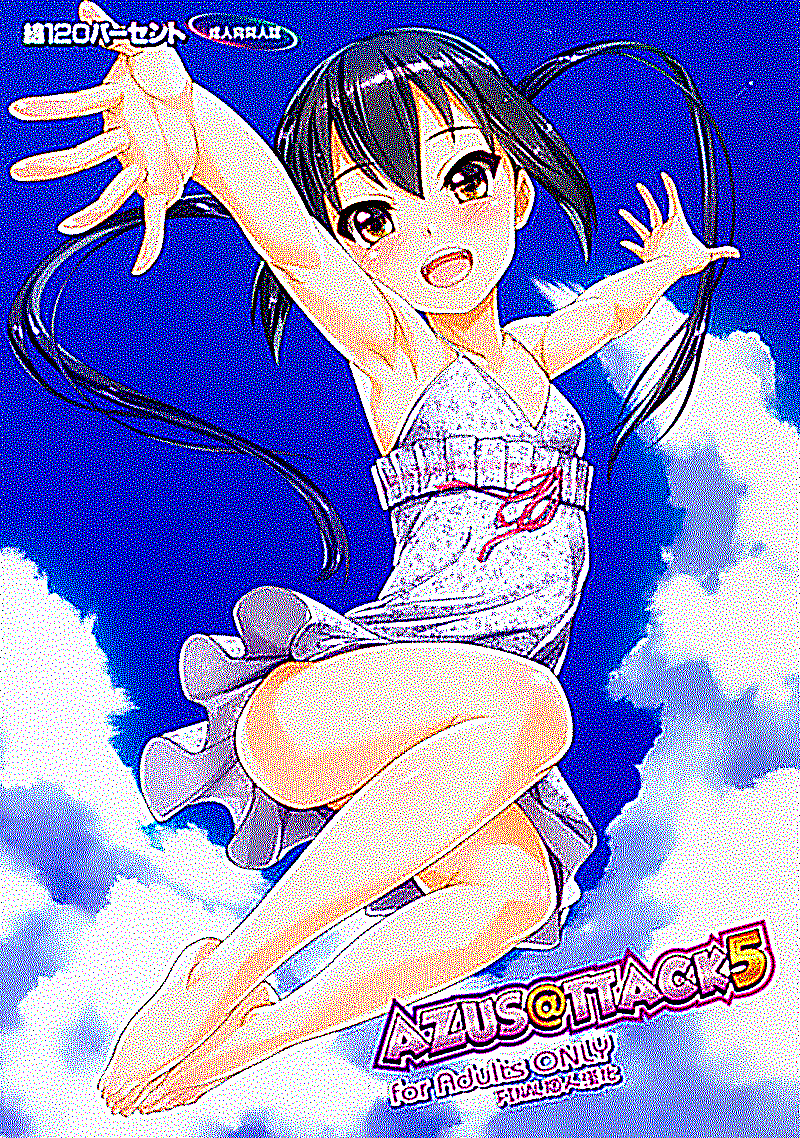
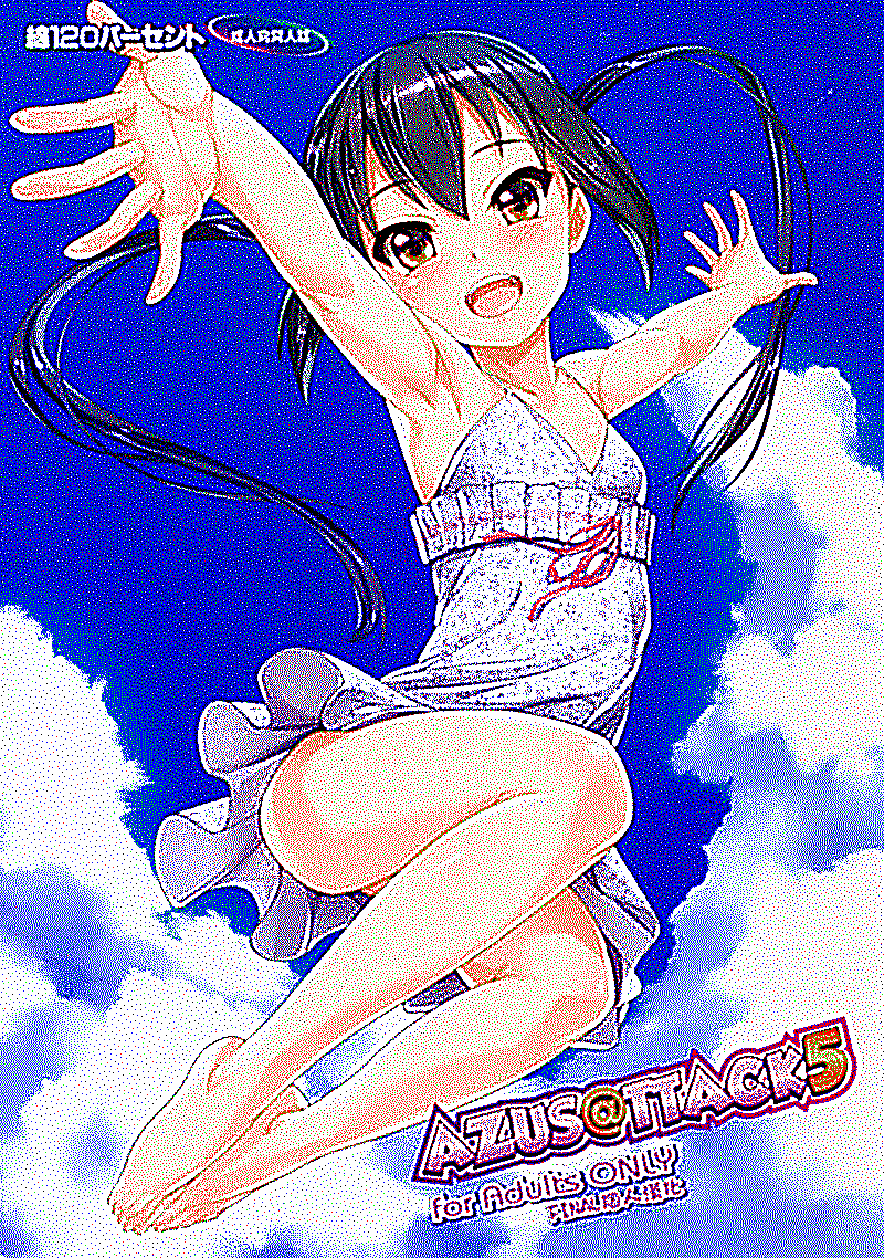
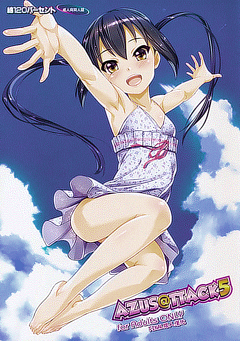
Available built-in CLI palettes are cube (the default, eight colors), rgbk
(red, green, blue, black), cmyk (white, black, yellow, magenta, cyan at
0.75 intensity), and bw (black and white). A JSON file can specify an
arbitrary nonempty list of normalized RGB triples, including fractional colors:
[
  [0.10, 0.15, 0.20],
  [0.85, 0.30, 0.20],
  [0.95, 0.90, 0.80]
]
uv run with-simple-color --input photo.png --palette palette.json --output halftone.npy
Use --show for an interactive comparison, or --comparison comparison.png
to save a two-panel comparison of the original and unblurred palette image.
Neither option displays a blurred image. --seed 0 is the CLI default.
--boundary, --init, --switch-fraction, and --tolerance expose optimization
settings; --quiet suppresses progress. --size changes the synthetic demo size.
All output paths must be distinct and must not overwrite an input image or palette.
Example outputs
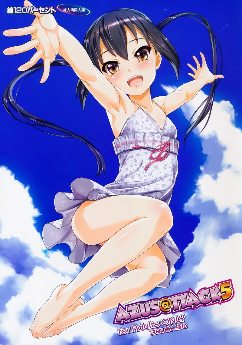
Unblurred palette halftones of the same image, rendered with the built-in palettes:
| Original | cube |
rgbk |
cmyk |
bw |
|---|---|---|---|---|
 |
 |
 |
 |
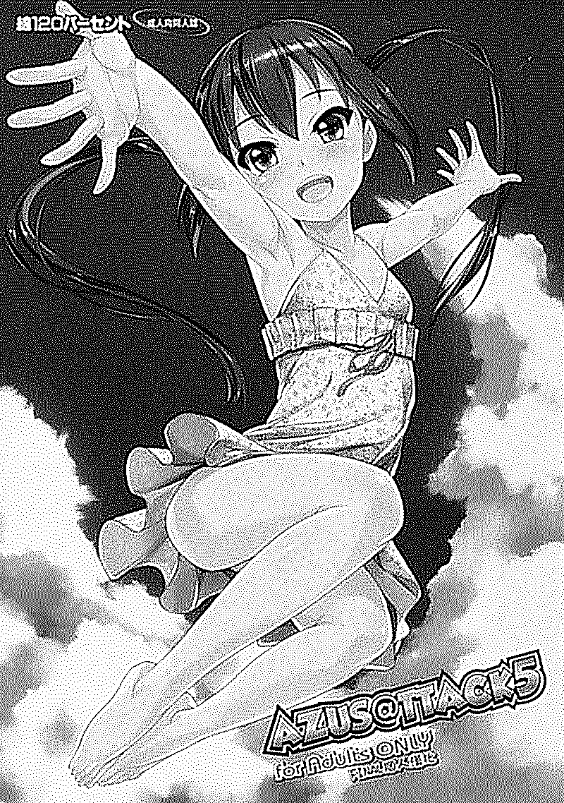 |
Image and color conventions
- The Python API and
.npyinputs require finite arrays of shape(height, width, 3)with values in[0, 1]. Integer 0/1 arrays are valid; divide 8-bit image arrays by 255 before calling the API. - Ordinary image files are loaded as 8-bit RGB, with EXIF orientation applied. Grayscale is expanded to RGB; transparency is composited over white.
- API results and
.npyoutputs arefloat64, preserving the supplied palette values after conversion tofloat64. Use.npyfor exact fractional colors. - PNG output rounds to 8-bit RGB. Fractional palette entries not representable
as multiples of
1/255cannot be preserved exactly in PNG. Reported loss refers to the in-memory result, before PNG rounding. - The objective operates in the supplied RGB coordinates. Image loading does not perform ICC color management or linear-light conversion. For a physical light-averaging model, convert both the image and palette to linear-light RGB before using the API, and apply the appropriate display conversion afterward.
Python API
import numpy as np

from with_simple_color import (
    compute_loss,
    quantize,
    validate_B_general,
)

image = np.full((32, 32, 3), 0.4)
palette = np.array([[0.0, 0.0, 0.0], [1.0, 1.0, 1.0]])
quantized, losses = quantize(
    image,
    sigma=2.0,
    palette=palette,
    max_iter=30,
    seed=42,
    verbose=False,
    return_history=True,
)
np.save("halftone.npy", quantized)
assert validate_B_general(quantized, palette)[0]
assert all(after <= before for before, after in zip(losses, losses[1:]))
print(compute_loss(quantized, image, sigma=2.0))
Without return_history=True, quantize returns only the unblurred image. The API's
default palette remains red, green, blue, and black, unlike the CLI demo's
eight-color palette. Existing helper names remain available from
with_simple_color.main and the package root. Use image= and quantized=
for named image arguments; the old positional argument order is unchanged.
Important options:
| Argument | Meaning |
|---|---|
sigma |
Finite positive Gaussian standard deviation in pixels. |
init="auto" |
Select the lower actual reconstruction loss of nearest-color and serpentine Floyd-Steinberg initializations. |
init="nearest" |
Start with the closest palette color at each pixel. |
init="error_diffusion" |
Use serpentine Floyd-Steinberg diffusion as a starting point, not as the optimizer. |
init="probabilistic" |
Sample distance-weighted palette colors. This is only a heuristic, not an unbiased color mixture. |
max_iter=30 |
Maximum sequential sweeps; zero returns the initialization unchanged. |
switch_fraction=1.0 |
Cap accepted changes per sweep at ceil(switch_fraction * height * width), in (0, 1]. Smaller values may need more sweeps. |
boundary_mode="reflect" |
reflect, mirror, nearest, wrap, or constant. Constant padding is zero; SciPy's grid aliases are also accepted by the API. |
seed=None |
Seed for random coordinate order and probabilistic initialization; set an integer for repeatability. |
tolerance=1e-12 |
Minimum absolute decrease in total squared error needed to accept one recoloring. |
return_history=False |
Return (quantized, losses) when true. History starts with the initialization loss. |
refine_general(quantized, image, sigma, palette, ...) improves an existing
palette image. Inputs are not mutated. plot_comparison(..., show=False)
returns a two-panel Matplotlib figure containing only the original and unblurred
palette image, suitable for saving without an interactive window. Plotting is
imported lazily; the internal reconstruction is not clipped before computing
the objective.
Objective and algorithm
Let image be the target and quantized[p] be one palette color at every pixel.
Let H be the spatial Gaussian blur, applied independently to each RGB channel.
The objective is:
minimize    L(quantized) = ||H(quantized) - image||_F^2
subject to  quantized[p] belongs to palette for every pixel p
The target is not blurred. H uses SciPy's discrete, normalized Gaussian
with truncate=4.0 and radius int(4 * sigma + 0.5), including the selected
boundary extension. The channel axis is never blurred.
For a recoloring at pixel p, define delta = new_color - old_color, the current
residual residual = H(quantized) - image, and column_p = H(unit_impulse_at_p).
Its exact change in loss is:
delta_loss = 2 * dot(delta, sum_over_pixels(column_p * residual))
             + dot(delta, delta) * sum_over_pixels(column_p ** 2)
The optimizer evaluates all palette colors for one pixel, accepts the best strictly improving choice, and immediately updates the residual before considering another pixel. This is discrete coordinate descent with exact single-pixel moves. It avoids treating overlapping pixel changes as independent.
Boundary-aware, sparse one-dimensional operator columns are constructed and
combined separably. Their squared norms depend on pixel position near edges;
they are not replaced by an infinite-domain kernel norm. This also avoids
incorrectly assuming that every boundary extension makes H self-adjoint.
No dense two-dimensional pixel-to-pixel blur matrix is constructed.
Each completed sweep recomputes the residual using SciPy. A sweep that fails
to reduce the measured objective is rolled back to protect against numerical
drift. Returned loss history therefore never increases. A full sweep with no
accepted changes certifies only that no single-pixel move improves the objective
by more than tolerance.
Limitations and cost
This is a discrete, nonconvex optimization problem. The implementation does
not promise the global minimum. It uses recolorings, not multi-pixel swaps;
escaping a one-pixel local optimum can require coordinated changes. Reaching
max_iter does not certify convergence. Different seeds and initializations
can yield different local solutions.
For normalized boundary modes, every reconstructed color is a convex combination
of palette colors. A target outside that convex hull cannot be reproduced
exactly. In particular, red/green/blue/black cannot represent white by spatial
mixing. The eight RGB cube corners span the full unit RGB cube, but spatial
coupling and discrete pixel counts still prevent arbitrary exact reconstruction.
Zero padding in constant mode additionally mixes black into border pixels.
With pixel_count = height * width, color_count palette colors, and Gaussian
radius radius, a sweep costs approximately
O(pixel_count * ((2 * radius + 1)**2 + color_count)). Large blur radii and
high-resolution images can be expensive; begin with a small image and a modest
sweep limit. Sparse operator construction uses
O((height + width) * (2 * radius + 1)) temporary storage, in addition to image
buffers and the palette. There is no height * width * color_count cost volume.
Development checks
uv run python -m compileall -q with_simple_color
uv run python -m with_simple_color --size 16 --max-iter 3 --output smoke.npy --comparison smoke.png
uv build
The numerical implementation can be independently checked by constructing each
Gaussian impulse with SciPy and comparing the predicted delta_loss with two
full objective evaluations. For tiny images, enumerate every recoloring after
convergence to verify one-pixel optimality. Check all five boundary modes,
singleton image dimensions, kernels larger than the image, fractional palettes,
and nonincreasing loss histories rather than judging only a displayed picture.
License
MIT. See LICENSE.
1 maintainer

Metadata
1 maintainer
Release files for with-simple-color 0.1.1
For a detailed explanation of source distributions (sdists) and built distributions (wheels), please see the package formats documentation.
Source distribution (sdist)
| File | Size | Uploaded | |
|---|---|---|---|
| with_simple_color-0.1.1.tar.gz | 16.7 kB | Details |
Built distribution (wheel)
| File | Interpreter | ABI | Platform | Reset |
|---|---|---|---|---|
| with_simple_color-0.1.1-py3-none-any.whl | Python 3 | none | any | Details |
Total release size: 32.0 kB
Release files / with_simple_color-0.1.1.tar.gz
| Download URL | with_simple_color-0.1.1.tar.gz |
|---|---|
| Size | 16.7 kB |
| Tags | Source |
|
SHA-256 checksum How to use checksums |
d0f552998af1b1a1c2ad6deb294d3ecf8784455ea01b91b1792863fface9d6e2
|
|
BLAKE2b-256 checksum How to use checksums |
49cd1194953ecf40ee0df3c064991d0106e4c0bd9430d6feb7b7bc855eb11b1a
|
| Upload date | |
|
Uploaded using Trusted Publishing? What is trusted publishing? |
No |
| Uploaded via |
poetry/2.4.1 CPython/3.14.6 Windows/11
|
Release files / with_simple_color-0.1.1-py3-none-any.whl
| Download URL | with_simple_color-0.1.1-py3-none-any.whl |
|---|---|
| Size | 15.3 kB |
| Tags | Python 3 |
|
SHA-256 checksum How to use checksums |
38592933e51d43f15eb502d53071528739e25893dd4ae7c3e13c83d7f5321d27
|
|
BLAKE2b-256 checksum How to use checksums |
8881d0240deb01fa404c0a31c419a45557db1cd861cba92e8c16f5ffc0a195b9
|
| Upload date | |
|
Uploaded using Trusted Publishing? What is trusted publishing? |
No |
| Uploaded via |
poetry/2.4.1 CPython/3.14.6 Windows/11
|














