
WKRLS — Wavelet Kernel-Based Regularized Least Squares



A Python library for estimating how the marginal effect of each regressor changes across time horizons — short, medium and long run — and across the distribution of the dependent variable, without assuming linearity or additivity.
Author: Dr Merwan Roudane · merwanroudane920@gmail.com · github.com/merwanroudane
What problem does this solve?
An ordinary regression gives you one number per regressor. That number is an average over two things that are usually not constant:
- Time horizon. A tax cut may stimulate output over two quarters and depress it over ten years. One coefficient reports a blend of the two and tells you neither.
- Position in the distribution. A variable may matter enormously in recessions and not at all in booms. A conditional-mean estimate averages that away.
WKRLS resolves both. It returns a marginal effect for every frequency band × every observation, and displays the result as a heatmap you can read at a glance.
It does this by composing two established methods:
| Component | Role | Reference |
|---|---|---|
| MODWT | Splits each series into components belonging to distinct time horizons | Percival & Walden (2000) |
| KRLS | Estimates a flexible conditional mean and returns a marginal effect for every observation | Hainmueller & Hazlett (2014) |
Installation
pip install git+https://github.com/merwanroudane/WKRLS.git
Or from a local clone:
git clone https://github.com/merwanroudane/WKRLS.git
cd WKRLS
pip install -e .
Requires Python 3.9+, numpy, pandas, scipy, statsmodels, matplotlib, PyWavelets. No compiler, no R, no MATLAB.
Sixty-second example
import wkrls as wk

data = wk.load_usmacro()                     # real US quarterly FRED data, bundled

res = wk.wkrls(
    y=data["realgdp"],
    X=data[["realcons", "realinv", "tbilrate"]],
    wavelet="la8", J=5,
)

res.summary()                                 # full estimation output
res.panel(colorscale="parula")                # the multi-panel heatmap
print(res.to_latex())                         # journal-ready LaTeX table
Output:
  band      variable                AME     Std.Err        z         p
  Short     realcons             0.65040    0.038974   16.688    0.0000 ***
  Short     realinv              0.13668   0.0058141   23.508    0.0000 ***
  Short     tbilrate          -0.0027984   0.0023552   -1.188    0.2348
  Medium    realcons             0.57546    0.025586   22.491    0.0000 ***
  ...
Consumption's effect on GDP is ≈ 0.65 in the short run — essentially its share in the national accounts, which is a reassuring sign the estimator is behaving.
The method, in three steps
        y, X  (stationary series, n observations)
          │
   ┌──────┴──────────────────────────────────────────────┐
   │ STEP 1   MODWT                                      │
   │ Decompose every series into detail levels D1…DJ,    │
   │ then group them into Short / Medium / Long bands.   │
   └──────┬──────────────────────────────────────────────┘
          │        one (y, X) pair per band
   ┌──────┴──────────────────────────────────────────────┐
   │ STEP 2   KRLS within each band                      │
   │ Gaussian kernel, λ by leave-one-out CV.             │
   │ Extract ∂y_i/∂x_ik for every observation i,         │
   │ then lowess-smooth them.                            │
   └──────┬──────────────────────────────────────────────┘
          │        smoothed effects, (bands × n × d)
   ┌──────┴──────────────────────────────────────────────┐
   │ STEP 3   Heatmap                                    │
   │ bands on the vertical axis, observations on the     │
   │ horizontal axis, effect as colour.                  │
   └─────────────────────────────────────────────────────┘
Step 1 — MODWT
The maximal overlap discrete wavelet transform splits a series into components associated with distinct periods. For quarterly data, detail level Dj carries oscillations of roughly 2^j to 2^(j+1) quarters:
| Band | Levels | Quarterly | Reading |
|---|---|---|---|
| Short | D1 + D2 | 2–8 quarters | business-cycle noise, transitory shocks |
| Medium | D3 + D4 | 8–16 quarters | the cycle proper |
| Long | D5 … DJ | 16+ quarters | structural, trend-like movements |
The MODWT is used rather than the ordinary DWT because it is shift-invariant (features stay aligned in time), it produces detail series the same length as the input (which is what makes a per-observation heatmap possible), and it is defined at any sample size.
Implementation note. This package implements the MODWT pyramid algorithm directly. It does not use
pywt.swt, which requires the sample length to be divisible by2^J— forn = 202, a perfectly ordinary quarterly sample,swtsilently permits onlyJ = 1. The decomposition here is verified in the test suite for additivity, energy preservation, shift-equivariance and frequency localisation at arbitraryn.
Step 2 — KRLS
Within each band, KRLS fits
$$ y_i = f(\mathbf{x}_i) + \varepsilon_i, \qquad f(\mathbf{x}) = \sum_j c_j \exp!\left(-\frac{\lVert \mathbf{x}-\mathbf{x}_j \rVert^2}{\sigma}\right) $$
with coefficients regularised by Tikhonov penalty:
$$ \mathbf{c}^* = (\mathbf{K}+\lambda \mathbf{I})^{-1}\mathbf{y} $$
and λ chosen by leave-one-out cross-validation (golden-section search on the closed-form LOO loss). The pointwise marginal effect for observation i and regressor k is available analytically:
$$ \frac{\partial \hat{y}i}{\partial x{ik}} = -\frac{2}{\sigma}\sum_j c_j K_{ij},(x_{ik}-x_{jk}) $$
That is one marginal effect per observation — not one per regressor.
Step 3 — Lowess and heatmap
Pointwise effects are noisy, so they are smoothed against the ordering variable with a lowess smoother (span 2/3 by default, matching R's lowess). The smoother is what you interpret, not the individual points.
Figures
Every figure is 300 dpi, serif-typeset, and returns a matplotlib Figure you can modify.
| Call | What you get |
|---|---|
res.panel() |
One heatmap panel per regressor — the main result figure |
res.heatmap(var) |
A single regressor's band × observation map |
res.pme_plot(var) |
Pointwise effects as dots with the lowess overlay |
wk.pme_grid(res) |
Every regressor's smoothed effect, lines by band |
res.surface_plot(var) |
3-D surface over (observation, band) |
res.contour_plot(var) |
Filled contours with labelled isolines |
res.forest_plot() |
Average marginal effects with 95% intervals |
wk.band_line_plot(res, var) |
Effect curves, one line per band |
wk.decomposition_plot(y, J=5) |
The MODWT decomposition itself |
wk.colorscale_preview() |
Swatches of every palette |
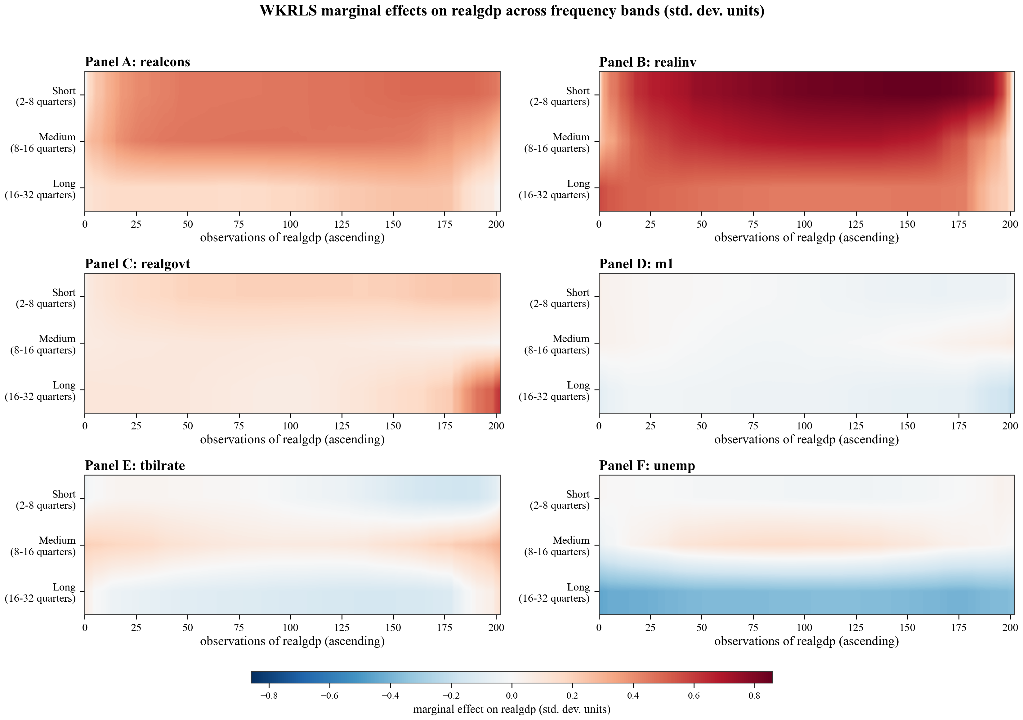
The main figure
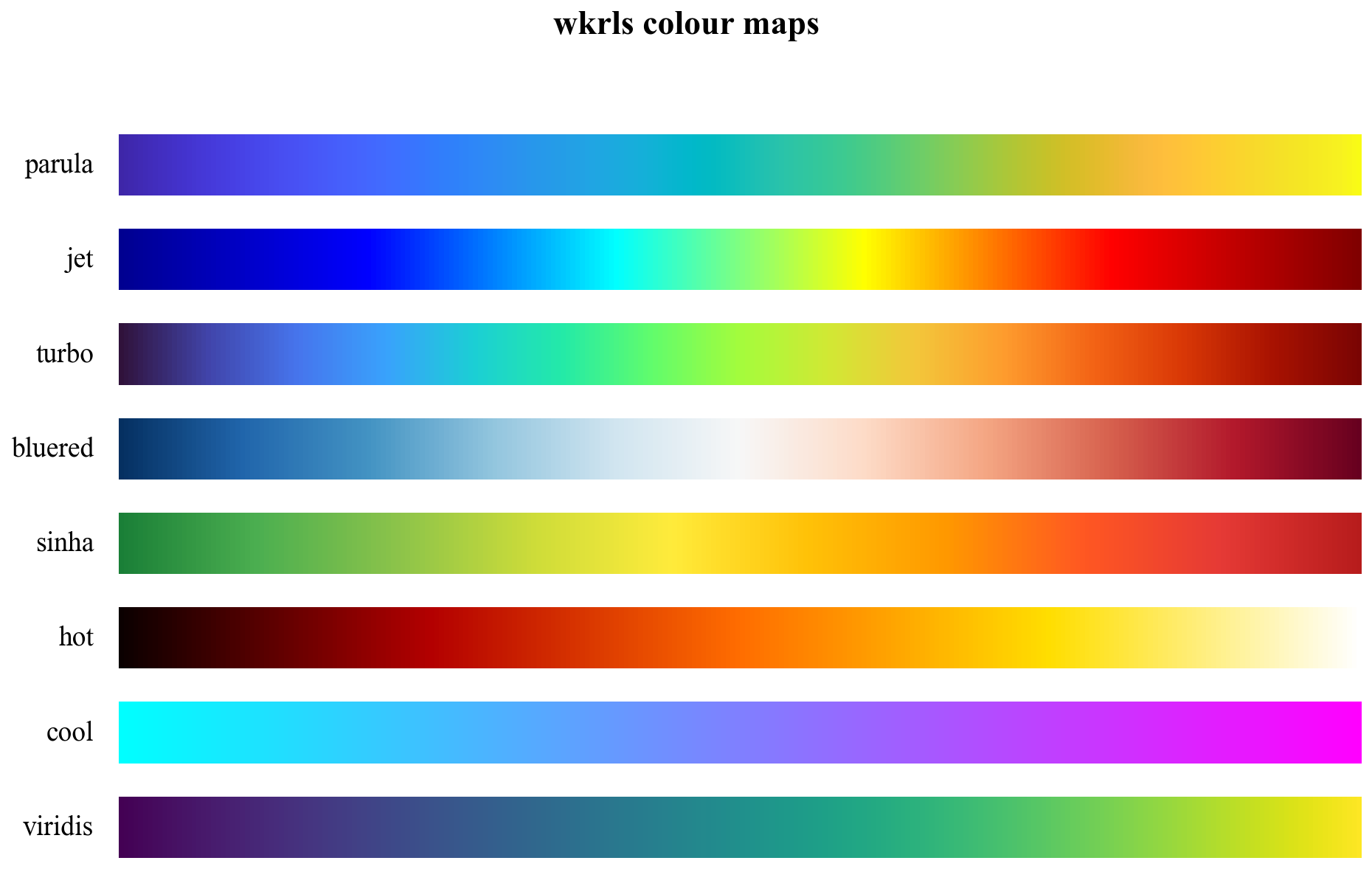
MATLAB colours
parula is the default, reproduced from the published 64 RGB stops of MATLAB R2014b — not an approximation.
res.panel(colorscale="parula")     # MATLAB R2014b default (package default)
res.panel(colorscale="jet")        # classic MATLAB rainbow
res.panel(colorscale="turbo")      # perceptually improved rainbow
res.panel(colorscale="bluered")    # diverging blue→red
res.panel(colorscale="sinha")      # diverging green→red
res.panel(colorscale="hot")        # MATLAB hot
res.panel(colorscale="cool")       # MATLAB cool
Palettes are also available as plain data:
wk.parula_colors(64)               # ['#3e26a8', '#4029b6', ...] hex list
wk.get_cmap("parula")              # matplotlib Colormap
wk.resolve_colorscale("Parula")    # plotly-style [(pos, hex), ...]
Making panels comparable
Raw marginal effects carry each regressor's own units, so putting six of them on one colour scale is misleading — a single large-magnitude regressor saturates the scale and flattens the rest. Two options:
res.panel()                                          # per-panel scale (default)
res.panel(shared_scale=True, standardize=True)       # one scale, unit-free
standardize=True multiplies each effect by sd(x_k)/sd(y) within the band, so a value of 0.4 reads "a one-standard-deviation rise in this regressor moves the dependent variable by 0.4 of its own standard deviations".
This changes the ranking in practice. In the six-variable US model shown above, investment's raw short-run effect (0.124) is far below consumption's (0.550) — but in standardised terms investment is larger (0.733 versus 0.431), because investment is so much more volatile that a typical move in it matters more for output. Both facts are true; they answer different questions, so report whichever matches the claim you are making.
Tables
print(res.to_latex())                      # booktabs, with \caption and \label
print(res.to_markdown())                   # for READMEs and notebooks
res.to_csv("results/")                     # every table in every format

wk.descriptives_latex(data)                # descriptive statistics
wk.diagnostics_latex(res)                  # per-band σ, λ, R², LOO error
wk.sign_summary_latex(res)                 # direction of each heatmap cell
LaTeX output uses booktabs rules with a tablenotes block carrying the significance legend. Add \usepackage{booktabs} to your preamble.
| Variable | Short | Medium | Long |
|---|---|---|---|
| realcons | 0.6504*** (0.0390) |
0.5755*** (0.0256) |
0.2475*** (0.0519) |
| realinv | 0.1367*** (0.0058) |
0.1182*** (0.0040) |
0.1488*** (0.0090) |
| tbilrate | -0.0028 (0.0024) |
0.0044*** (0.0012) |
0.0074*** (0.0009) |
Diagnostics
Two questions decide whether WKRLS suits your data:
report = wk.diagnostic_report(data)
- Are the series non-normal? — descriptive statistics with skewness, excess kurtosis and Jarque–Bera. Heavy tails weaken the case for linear-Gaussian estimation.
- Is the dependence nonlinear? — the BDS test (Broock, Scheinkman, Dechert & LeBaron 1996). KRLS is a nonparametric estimator; if the data are i.i.d. or linearly dependent, its flexibility buys nothing and a linear model is more efficient. Rejection of the i.i.d. null across embedding dimensions is the standard justification for reaching for a kernel method.
Stationarity testing is deliberately not included — it is a property of your data pipeline rather than of WKRLS, and statsmodels already provides adfuller, kpss and friends. Stationarise before estimating; wk.log_diff is provided for the usual case.
Estimation choices, and why they are yours to make
WKRLS was introduced in an applied paper that describes the method in a three-step recipe without a formal derivation. Several choices are therefore not settled by the source, and this package exposes each one as an argument with a documented default rather than burying a silent decision.
| Choice | Default | Alternative | Does it move the estimates? |
|---|---|---|---|
wavelet |
"la8" |
any orthogonal filter | Yes — check robustness |
J, band_spec |
5, Short/Medium/Long |
any grouping | Yes |
multivariate |
True — all regressors enter one KRLS jointly, so each effect is conditional on the others |
False — a separate bivariate fit per regressor |
Yes, substantially |
order_by |
"y" — effects indexed against the dependent variable |
"x" — against each regressor's own values |
No (surface only) |
lowess_frac |
2/3 (R's lowess default) |
any span in (0, 1] | No (surface only) |
sigma, lambda_ |
d, and LOO-CV per band |
user-supplied | Yes |
The multivariate choice matters most. The source paper does not state which it used; this package defaults to the joint fit because that is what KRLS is designed for and what the applied KRLS literature does, but the bivariate reading is one keyword away.
Report robustness. Example 2 includes a ready-made grid:
                                   realcons/Short  realcons/Long  unemp/Long
baseline (la8, J=5, multivariate)          0.5502         0.2201     -0.0464
wavelet d4                                 0.5543         0.4278     -0.0305
wavelet la16                               0.5634         0.5632      0.0159
wavelet haar                               0.5610         0.3416     -0.0364
J = 3                                      0.5641         0.5821      0.0146
bivariate KRLS                             0.4232         1.0490     -0.1142
reflection boundary                        0.5545         0.4619     -0.0445
eigtrunc 0.001                             0.4223         0.2121     -0.0437

Sign stable across all 8 specifications in 5/6 cells.
Sign-unstable cells: ['unemp/Long']
Read that honestly: consumption's short-run effect is rock-solid (0.42–0.56 everywhere), its long-run effect is sign-stable but varies by a factor of five, and unemployment's long-run effect flips sign under two specifications — so it is not a finding, and should be reported as sensitive to the wavelet choice rather than claimed.
Inference
The source method reports no standard errors. This package computes them from the KRLS variance of the average derivative and labels them as an addition:
res.ame       # ame, std_error, z_value, p_value, stars, ame_std, share_positive
res.forest_plot(alpha=0.05)
These apply to the average marginal effect within a band. There is no pointwise inference on the heatmap surface itself — if you need it, bootstrap over the estimation.
API reference
Estimation
wk.wkrls(y, X, wavelet="la8", J=5, bands=True, band_spec=None,
         multivariate=True, order_by="y", lowess_frac=2/3, lowess_it=3,
         sigma=None, lambda_=None, eigtrunc=None, boundary="periodic",
         freq="quarterly", dep_name=None, var_names=None, verbose=True)
WKRLSResult
| Attribute | Type | Contents |
|---|---|---|
.bands, .var_names, .dep_name, .n |
model structure | |
.derivatives[band] |
(n, d) |
raw pointwise marginal effects |
.smoothed[band] |
(n, d) |
lowess-smoothed effects — the heatmap payload |
.ame |
DataFrame | average effects with inference, per (band, variable) |
.diagnostics |
DataFrame | per-band σ, λ, R², LOO error |
.fits[band] |
KRLSResult |
the underlying KRLS fit |
.band_sd_x, .band_sd_y |
standardisation weights |
Methods: .summary(), .to_matrix(var), .surface(var), .effects_frame(), .sign_summary(), .to_latex(), .to_markdown(), .to_csv(path), plus every plotting shortcut.
Standalone KRLS
The KRLS engine is a faithful port of the R package KRLS 1.1-0 and is usable on its own:
fit = wk.krls(X, y)                # Gaussian kernel, λ by LOO-CV
fit.derivatives                    # (n, d) pointwise marginal effects
fit.ame_table()                    # averages with inference
fit.predict(new_X)
Validated in the test suite against a linear DGP (recovers the true slopes), a nonlinear DGP (correlation 0.98 with the true pointwise derivative), and central finite differences (agreement to 1e-4).
Wavelets, colours, data
wk.modwt_mra(x, "la8", J=5)              # ([D1..DJ], SJ)
wk.decompose_frame(df, J=5)              # {band: DataFrame}
wk.max_modwt_level(n, "la8")             # largest sensible J

wk.parula_colors(n) / matlab_jet_colors / turbo_colors
wk.bluered_colors / sinha_colors / hot_colors / cool_colors
wk.get_cmap(name) / resolve_colorscale(name) / list_colorscales()

wk.load_usmacro()                        # real FRED data, bundled
wk.simulate_wkrls(n=256, seed=0)         # known frequency-varying structure
Bundled data
usmacro — US quarterly macroeconomic aggregates, 1959Q1–2009Q3 (n = 203), from the Federal Reserve Economic Data (FRED) service of the Federal Reserve Bank of St. Louis, distributed with statsmodels. Public domain. Twelve series: real GDP, consumption, investment, government spending, disposable income, CPI, M1, the T-bill rate, unemployment, population, inflation and the real interest rate.
wk.load_usmacro()                                  # 7-series working set, log-differenced
wk.load_usmacro(transform=None)                    # levels
wk.load_usmacro(columns=["realgdp", "cpi", "m1"])  # your own selection
Examples
| Script | What it demonstrates |
|---|---|
examples/01_quickstart.py |
A complete analysis in twenty lines |
examples/02_full_study.py |
Paper-shaped workflow: raw data → diagnostics → estimation → robustness grid → exported figures and tables |
examples/03_validation.py |
Recovers a planted frequency-varying structure, and shows what OLS misses |
python examples/02_full_study.py
A step-by-step tutorial that builds the analysis one line at a time is in GUIDE.md.
Testing
pytest tests -q                        # 72 tests
pytest --doctest-modules wkrls -q      # 16 doctests
The suite checks the MODWT (additivity, energy, shift-equivariance, frequency localisation at awkward sample sizes), the KRLS engine (recovery of known effects, agreement with finite differences, derivative sign), the WKRLS pipeline (structure, recovery of a planted structure, placebo behaviour), every figure, and the BDS test against both i.i.d. noise and a chaotic map.
Citation
@software{roudane_wkrls_2026,
  author  = {Roudane, Merwan},
  title   = {{WKRLS}: Wavelet Kernel-Based Regularized Least Squares for Python},
  year    = {2026},
  version = {1.0.0},
  url     = {https://github.com/merwanroudane/WKRLS}
}
Please also cite the underlying methods:
- Adebayo, T. S., Eweade, B. S., Özkan, O. & Uzun Ozsahin, D. (2025). Effects of energy security and financial development on load capacity factor in the USA: a wavelet kernel-based regularized least squares approach. Clean Technologies and Environmental Policy, 27, 4215–4232. doi:10.1007/s10098-024-03109-1
- Hainmueller, J. & Hazlett, C. (2014). Kernel Regularized Least Squares: Reducing Misspecification Bias with a Flexible and Interpretable Machine Learning Approach. Political Analysis, 22(2), 143–168. doi:10.1093/pan/mpt019
- Percival, D. B. & Walden, A. T. (2000). Wavelet Methods for Time Series Analysis. Cambridge University Press.
- Broock, W. A., Scheinkman, J. A., Dechert, W. D. & LeBaron, B. (1996). A test for independence based on the correlation dimension. Econometric Reviews, 15(3), 197–235. doi:10.1080/07474939608800353
License
MIT — see LICENSE.
1 maintainer

Metadata
1 maintainer
Release files for wkrls 1.0.0
For a detailed explanation of source distributions (sdists) and built distributions (wheels), please see the package formats documentation.
Source distribution (sdist)
| File | Size | Uploaded | Provenance | |
|---|---|---|---|---|
| wkrls-1.0.0.tar.gz | 73.5 kB | Without provenance | Details |
Built distribution (wheel)
| File | Interpreter | ABI | Platform | Reset |
|---|---|---|---|---|
| wkrls-1.0.0-py3-none-any.whl | Python 3 | none | any | Details |
Total release size: 138.0 kB
Release files / wkrls-1.0.0.tar.gz
| Download URL | wkrls-1.0.0.tar.gz |
|---|---|
| Size | 73.5 kB |
| Tags | Source |
|
SHA-256 checksum How to use checksums |
cf8d234baa9c0c0aba8f31ae48416756f97633cef6db17ad5402cb0a51845f65
|
|
BLAKE2b-256 checksum How to use checksums |
7707f5fac890bd73cdb8432dbbc7048ccb38af55db08ec2ec0eb493b9ef4f9ef
|
| Upload date | |
|
Uploaded using Trusted Publishing? What is trusted publishing? |
No |
| Uploaded via |
twine/7.0.0 CPython/3.11.0
|
Release files / wkrls-1.0.0-py3-none-any.whl
| Download URL | wkrls-1.0.0-py3-none-any.whl |
|---|---|
| Size | 64.5 kB |
| Tags | Python 3 |
|
SHA-256 checksum How to use checksums |
af5597f67497c51d2483420d3b11aad4092a9734207197fb4f0c2000e7623653
|
|
BLAKE2b-256 checksum How to use checksums |
66561a401fbf9fdc87453021ea86e4b71dd9d6084208b47d78255781956a7a83
|
| Upload date | |
|
Uploaded using Trusted Publishing? What is trusted publishing? |
No |
| Uploaded via |
twine/7.0.0 CPython/3.11.0
|
Security for wkrls 1.0.0
Provenance
Provenance describes where a file came from. On PyPI, provenance is shared via attestations, which provide a verifiable record of the build or publishing details. View details, limitations and caveats.
No provenance found
None of the files in this release were uploaded with provenance metadata.
A note on package security
PyPI is a repository for distributing packages, not a service for auditing them. While third-party security researchers and our staff do their best to detect and remove malicious packages, PyPI cannot guarantee the quality, security or suitability of any given package.
To learn more about protecting yourself from malicious actors, visit our package security documentation.













